Predicting High School Graduation From Kindergarten Data. Hyperparameter tuning (part 2)

Random Forest

A simple but very effective improvement on basic decision trees is run many of them on samples with replacement from the original training set and take the average. This is called bagging. We already did bagging of sorts in that we fit five different regression trees on the five cross validation data sets and took the mean. With random forest, we randomly sample with replacement from the data set many more, say 1000, times. Moreover, when making a cut, the random forest algorithm no longer considers all k dimensions (of the k features/predictors), but a smaller number of d dimensions. The standard value of this parameter d, which is called mtry in the ranger engine we will use, is the square root of k, rounded up. It works very well in practice, but we will see if we can improve on it a bit by tuning it.

The big question we want to answer first however, is why one would ever want to use fewer dimensions in cutting up the space in which the predictors and outcomes live. The reason is that if there were a very strong predictor, it would dominate all of the 1000 runs. In that case, there is not much information added by averaging over the 1000 trees. The runs are too similar. By randomly selecting features, it is ensured that new information in brought to the table, while random mistakes in classification cancel out when taking the average.

We will now run the random forest algorithm for a number of minimal points per node and variables considered (mtry). We specify that we want to tune these parameters in the model setup.

star_forest <- rand_forest(
  mtry = tune(),
  trees = 1000,
  min_n = tune() ) %>%
    set_mode("classification") %>%
    set_engine("ranger")

# Create custom metrics function
star_metrics <- metric_set(accuracy, roc_auc, sens, spec)

We then tune using 20 points in the grid. We tune on the five folds that we set up earlier. That way we are less likely to overfit and get different results when we apply the trained model to the test set.

# Set up the workflow
star_wkflw <- workflow() %>% 
  add_recipe(star_rec)

randfor_wf <- star_wkflw %>% 
  add_model(star_forest) 

doParallel::registerDoParallel()
set.seed(111)
tune_forest <- tune_grid(
  randfor_wf,
  resamples = star_folds,
  grid=20,
  control= control_grid(save_pred = T),
  metrics = star_metrics
)

tune_forest %>% 
  collect_metrics() 

## # A tibble: 80 x 8
##     mtry min_n .metric  .estimator  mean     n std_err .config              
##    <int> <int> <chr>    <chr>      <dbl> <int>   <dbl> <chr>                
##  1    15    15 accuracy binary     0.722     5  0.0110 Preprocessor1_Model01
##  2    15    15 roc_auc  binary     0.695     5  0.0131 Preprocessor1_Model01
##  3    15    15 sens     binary     0.808     5  0.0118 Preprocessor1_Model01
##  4    15    15 spec     binary     0.426     5  0.0113 Preprocessor1_Model01
##  5    59    40 accuracy binary     0.718     5  0.0100 Preprocessor1_Model02
##  6    59    40 roc_auc  binary     0.680     5  0.0144 Preprocessor1_Model02
##  7    59    40 sens     binary     0.806     5  0.0115 Preprocessor1_Model02
##  8    59    40 spec     binary     0.413     5  0.0149 Preprocessor1_Model02
##  9    22    28 accuracy binary     0.720     5  0.0110 Preprocessor1_Model03
## 10    22    28 roc_auc  binary     0.690     5  0.0130 Preprocessor1_Model03
## # ... with 70 more rows

We pull out 20 times the four metrics that we specified. Results look quite similar to the logistic regression, although the specificity is lower. There is some variation in the values between parameter specifications. Let’s plot these with regard to the roc_auc.

tune_forest %>% 
  collect_metrics() %>% 
  filter(.metric == "roc_auc") %>% 
  pivot_longer(min_n:mtry, values_to = "value", names_to = "parameter") %>% 
  ggplot(aes(value,mean, color=parameter)) +
  geom_point(show.legend = F) +
  facet_wrap(~ parameter, scales= "free_x") +
  theme_minimal()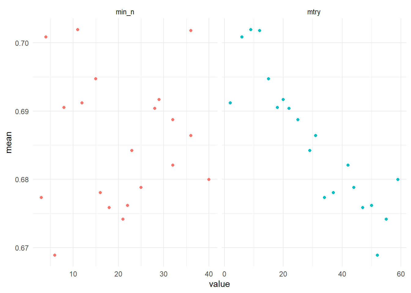

For the minimal points per node (min_n) parameter there is no clear relation between its size and the roc_auc, but lower numbers of the number of variables considered on which to make split (mtry) perform better. We pick some sensible ranges for both parameters to see if we can squeeze out some performance gain by tuning a second time.

rf_grid <- grid_regular(
  min_n(range = c(10,35)),
  mtry(range=c(1,10)),
  levels=5
)

tune_forest_manual <- tune_grid(
  randfor_wf,
  resamples = star_folds,
  grid=rf_grid,
  control= control_grid(save_pred = T)
)

tune_forest_manual %>% 
  collect_metrics() %>% 
  filter(.metric=="roc_auc") %>% 
  mutate(min_n = factor(min_n)) %>% 
  ggplot(aes(mtry, mean, color=min_n)) + 
  geom_line(alpha=0.4, size=1.2) +
  geom_point()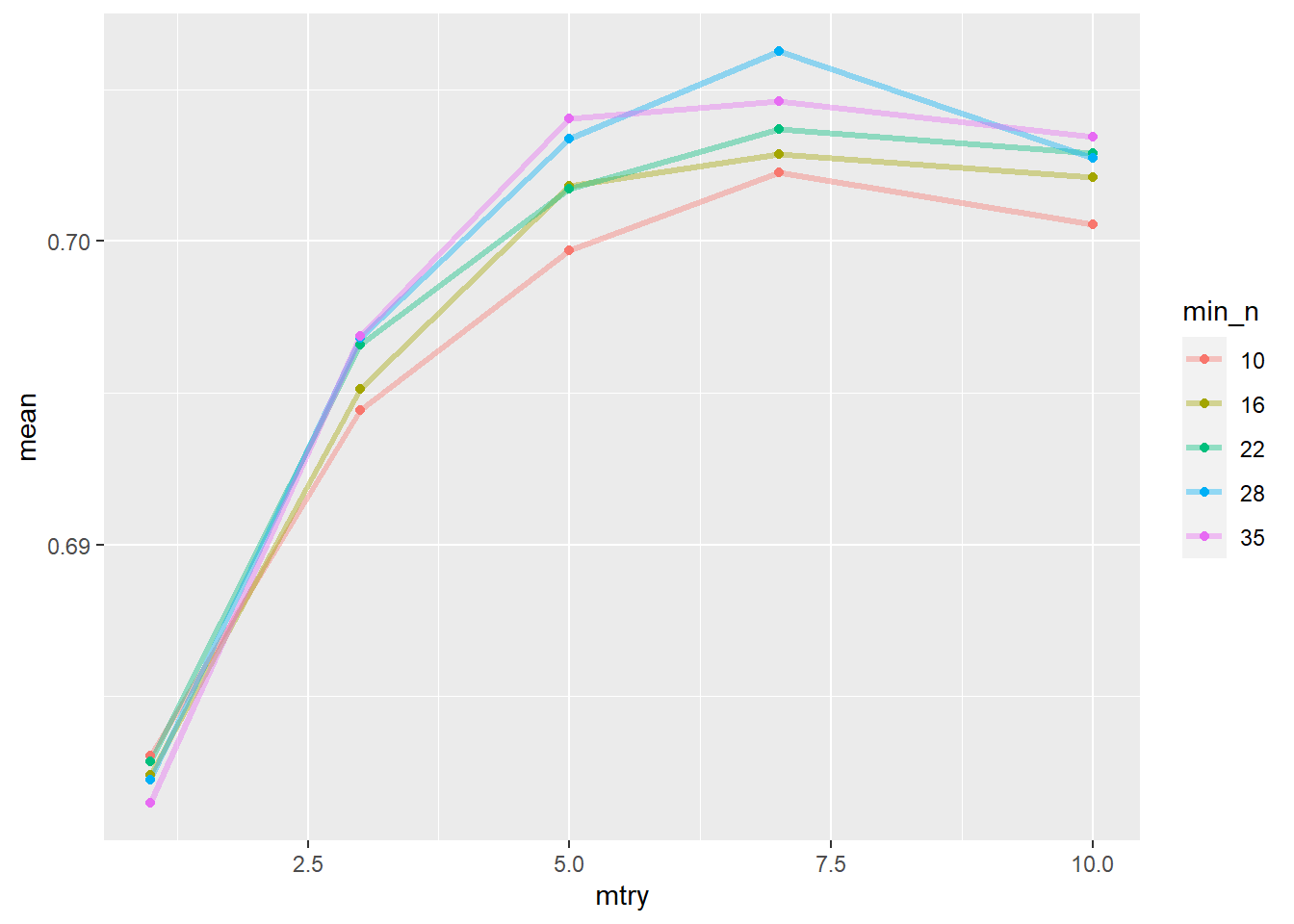

The splot suggests mtry around 7 and min_n of 28 is optimal. Let’s confirm this.

best_auc <- select_best(tune_forest_manual, "roc_auc")

best_auc

## # A tibble: 1 x 3
##    mtry min_n .config              
##   <int> <int> <chr>                
## 1     7    28 Preprocessor1_Model19

We now plug these parameter values into the model and apply it to the test data with the last_fit function of tidymodels.

final_rf <- finalize_model(
  star_forest,
  best_auc
)

final_wf <- workflow() %>% 
  add_recipe(star_rec) %>% 
  add_model(final_rf)

final_res <- final_wf %>% 
  last_fit(star_split,
           metrics = star_metrics)

final_res %>% collect_metrics()

## # A tibble: 4 x 4
##   .metric  .estimator .estimate .config             
##   <chr>    <chr>          <dbl> <chr>               
## 1 accuracy binary         0.764 Preprocessor1_Model1
## 2 sens     binary         0.836 Preprocessor1_Model1
## 3 spec     binary         0.513 Preprocessor1_Model1
## 4 roc_auc  binary         0.761 Preprocessor1_Model1

The results on the test set are a little bit lower than on the training set, but not much. They are similar to the logistic model, but the specificity is lower. Let’s also plot the roc curve, which tells the same story graphically, but adds information in what different thresholds within the nodes would accomplish.

final_res %>% 
  collect_predictions() %>% 
  roc_curve(hsgrdcol, .pred_YES) %>% 
  autoplot()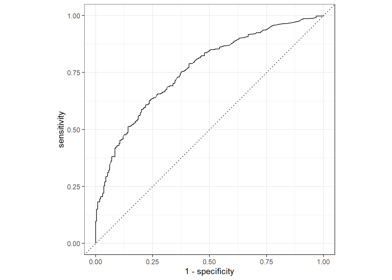

So far, we let decision tree algorithms make cuts in the data by looking at an impurity measure. We have no idea how they did so. It would be interesting though to at least know which features were important in making the prediction.

One way to do so is to track for every feature by how much it brought down the impurity on average. It turns out though that this method inflates the importance of continuous features and so introduces bias. A remedy is to permute the columns values of a feature and rerun the random forest. The drop in accuracy compared to the initial model is then attributed to the feature.

tree_prep <- prep(star_rec)

final_rf %>% 
  set_engine("ranger", importance="permutation") %>% 
  fit(hsgrdcol ~ .,
      data = juice(tree_prep)) %>% 
  vip(geom="point")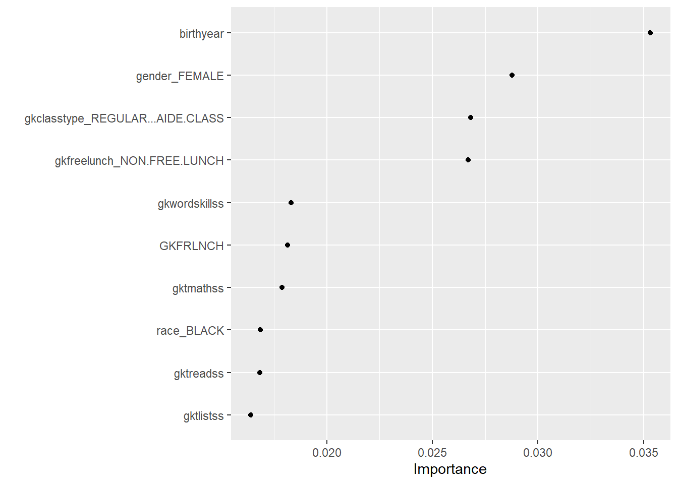

The influence of birth year is surprising and not immediately clear. Whether a student receives a free lunch or not gives information on the social economic status of the parents and makes sense. The variable ‘Regular class’ gives information on class size. Interestingly, the algorithm makes ample use of teacher attributes (gkt stands for group kindergarten teacher), which suggests teachers play an important role.

Boosting

Another way to enhance the quality of the predictions of decision trees is to boost them. The technique of gradient boosting is quite elegant. It chains weak learners (such as decision trees that predict barely better than chance) together, so that they become a strong predictor. It does so by taking tiny steps. At every step, the residual of the prediction and the outcome label is used to extend the overall prediction in the right direction. The size of these steps is controlled by the learning rate parameter.

We use the XgBoost algorithm, which also has a loss reduction hyperparameter. It sets a bar for the amount of gain we must make at each step towards the outcome label. If a step doesn’t achieve this level, the algorithm prunes it away.

We set of the XgBoost formula and the grid for training the hyperparameters.

boost_tune_spec <- boost_tree(
  trees=1000,
  tree_depth=tune(), min_n=tune(), loss_reduction=tune(),
  sample_size=tune(), mtry=tune(), learn_rate=tune() ) %>% 
  set_engine('xgboost') %>% 
  set_mode("classification")

xgb_grid <- grid_latin_hypercube(
  tree_depth(), 
  min_n(), 
  loss_reduction(), 
  sample_size=sample_prop(), 
  finalize(mtry(), star_train),
  learn_rate(),
  size=20
)

We then run the model for the hyperparameters in this grid and plot the results.

xgb_workflow <- workflow() %>% 
  add_recipe(star_rec) %>% 
  add_model(boost_tune_spec)

doParallel::registerDoParallel()

set.seed(112)
xbg_res <- tune_grid(
  xgb_workflow,
  resamples=star_folds,
  grid=xgb_grid,
  control= control_grid(save_pred = T)
)

xbg_res %>% 
  collect_metrics() %>% 
  filter(.metric=="roc_auc") %>% 
  select(mean,mtry:sample_size) %>% 
  pivot_longer(mtry:sample_size, names_to="parameter", values_to="value") %>% 
  ggplot(aes(value, mean, color=parameter)) +
  geom_point(legend=F) +
  facet_wrap(~ parameter, scales="free_x") +
  theme_minimal()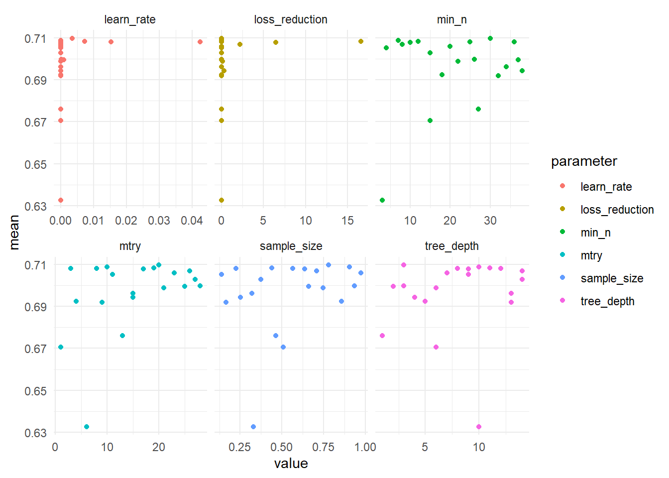

On the y-axis is the mean area under the roc-curve, while the x-axis displays values of the hyperparameter that is tuned. No clear patterns emerge, besides that fact that the model doesn’t fare well if the hyperparameters are too low.

We select the model with the hyperparameters that maximize the area under the roc curve. Let’s draw the roc curve for our final fit, which applies the model to the test set (we can get a rough idea of the performance of the XgBoost model on the training set by glancing the y-axis of the plot above).

set.seed(124)
best_auc <- select_best(xbg_res, "roc_auc")
final_xgb <- finalize_workflow(xgb_workflow, best_auc)
final_res <- last_fit(final_xgb, 
                      star_split,
                      metrics = star_metrics) 
final_res %>% collect_predictions() %>% 
  roc_curve(truth=hsgrdcol,.pred_YES) %>% 
    autoplot()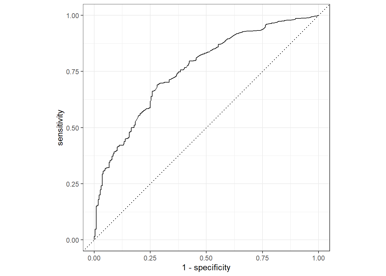

To get a better understanding of the meaning of this curve, we print out some of the thresholds that determine whether an observation is labeled YES (graduation) or NO (drop out).

final_res %>% collect_predictions() %>% 
  roc_curve(truth=hsgrdcol,.pred_YES) %>% 
  arrange(desc(.threshold))

## # A tibble: 715 x 3
##    .threshold specificity sensitivity
##         <dbl>       <dbl>       <dbl>
##  1    Inf               1     0      
##  2      0.918           1     0.00129
##  3      0.916           1     0.00258
##  4      0.915           1     0.00387
##  5      0.914           1     0.00516
##  6      0.913           1     0.00645
##  7      0.912           1     0.00774
##  8      0.911           1     0.00903
##  9      0.910           1     0.0103 
## 10      0.908           1     0.0116 
## # ... with 705 more rows

If we wanted to catch all drop outs, we pick a threshold of about 94%. This corresponds to a point on the bottom left of the curve. That would mean simply labeling almost all the points as NO (as the corresponding sensitivity tells us). We would manually pick a threshold that satisfied the needs of the practical situation. As this is a theoretical exercise, we won’t bother with this. The standard 0.5 threshold gives us the table below.

final_res %>% 
  collect_metrics()

## # A tibble: 4 x 4
##   .metric  .estimator .estimate .config             
##   <chr>    <chr>          <dbl> <chr>               
## 1 accuracy binary         0.720 Preprocessor1_Model1
## 2 sens     binary         0.750 Preprocessor1_Model1
## 3 spec     binary         0.616 Preprocessor1_Model1
## 4 roc_auc  binary         0.759 Preprocessor1_Model1

We didn’t outperform the logistic regression by much, which is slightly disappointing.

final_res %>% collect_predictions() %>% 
  conf_mat(hsgrdcol, .pred_class)

##           Truth
## Prediction YES  NO
##        YES 581  86
##        NO  194 138

The confusion matrix on the test set (which contains fewer observations than the ones we showed in the previous post) gives us a feel for what it would mean to apply this algorithm in the real world. Out of the over 200 eventual high school drop outs, we would pick out over 100 with our algorithm, at the cost of also selecting 200 pupils that would graduate anyway.

star_prep <- prep(star_rec)

final_xgb %>%
  fit(data = star_train) %>%
  pull_workflow_fit() %>%
  vip(geom = "point")

## [19:21:04] WARNING: amalgamation/../src/learner.cc:1095: Starting in XGBoost 1.3.0, the default evaluation metric used with the objective 'binary:logistic' was changed from 'error' to 'logloss'. Explicitly set eval_metric if you'd like to restore the old behavior.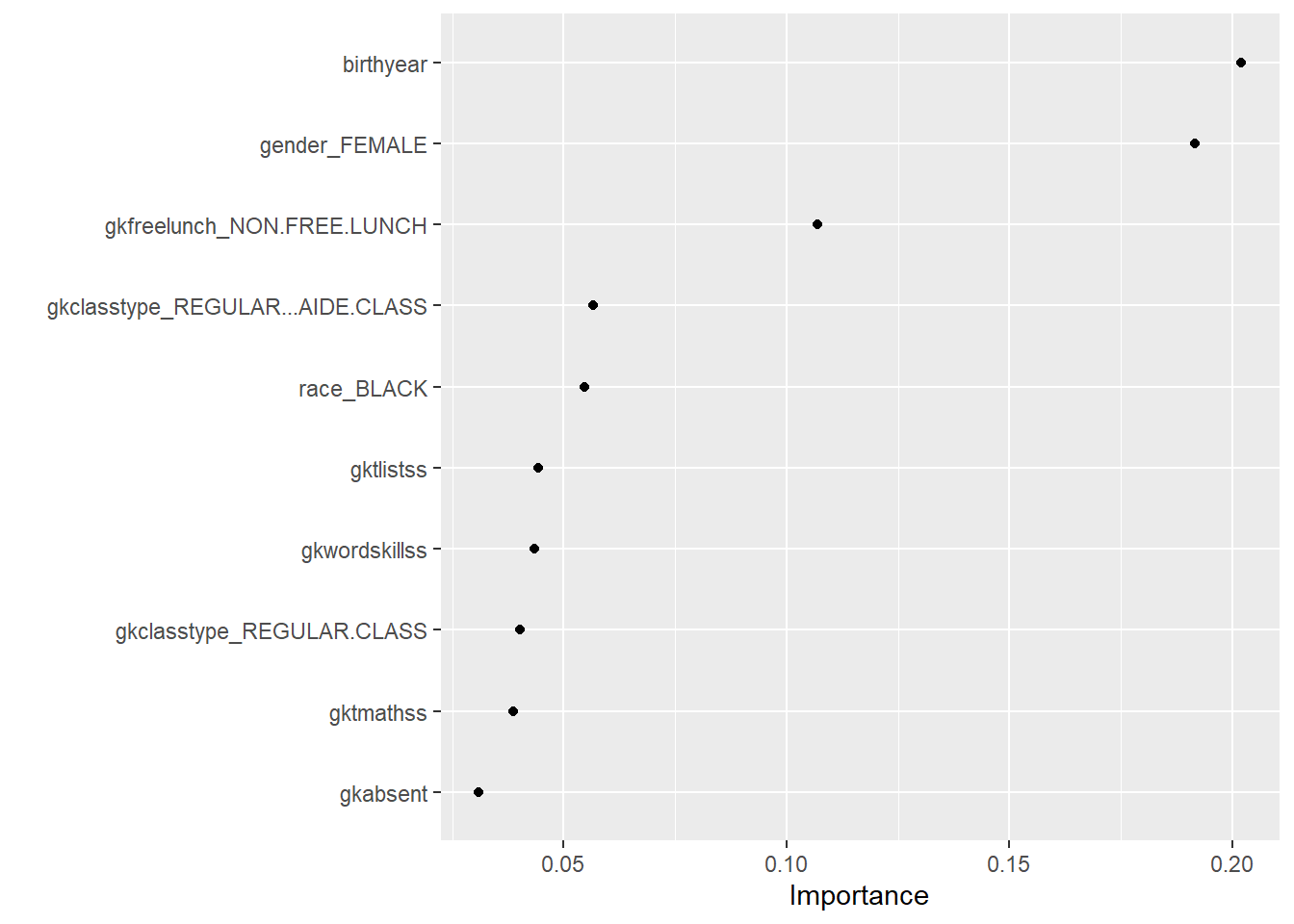

The features used by the XgBoost algorithm are very similar to those used by the Random Forest algorithm.