Predicting High School Graduation From Kindergarten Data. Basic Decision Trees (part 1)
In ever more domains of life experts have to compete with algorithms when they make predictions. Almost always, the experts mistrust algorithmic predictions. However, the work of Meehl, Kahneman and others suggests that it is hard to find evidence of expert judgments trumping even simple algorithms. Especially if the expert does not receive clear feedback of his or her predictions.
In the context of education, the problem props up when students have to be classified so that their education is tailored to their ‘level’. In the Dutch system this classification happens relatively early, as students are already placed into a stream at the end of primary school. A long standing debate is about whether this decision should be based on test scores, teacher judgment or a mix of the two.
Evidence suggests the picture is mixed, but that teachers may on average do a little better than the threshold based on a test score. Beating an algorithm that takes in one number is nothing to be too proud of though. In this post I therefore want to explore how accurately one can predict student achievement if more predictors (or ‘features’ in the machine learning lingo) are considered. I do not have access to such data from the Dutch education system, but I do have access to data from the US, which allows one to a make related predictions.
Specifically, the challenge I set myself in this post is to predict who will graduate high school and who will drop out, by looking at data about kids in kindergarten (5-7 years old). The practical use of this analysis is not hard to see: if we can identify those at risk of dropping out at an early age more accurately, we can allocate pedagogical resources more efficiently to those who need them most.
A next step would be to compare such predictions to those of experts, which were unfortunately not measured and recorded in this data set.
After briefly exploring the data, we fit a basic decision tree and a logistic model. In a follow up post we attempt to tweak the decision tree by means of bagging and boosting, so that it can hopefully beat the logistic model.
The Data
We will use data from the famous STAR study that was carried out in Tennessee from 1985 onward. The study took the form of a massive randomized controlled trial with over 10 000 kids, in which kids in kindergarten were randomly assigned to classrooms of different sizes. This treatment was continued for another three years. To date, the study still provides the best experimental evidence of the causal impact of reduced class size source. We don’t care about class size for the purpose of this project of course, and only care about the data because it measured so many variables and because is has since been recorded whether the participants graduated from high school.
There are too many variables to discuss here. Basic variables like gender, race and birth month are recorded, as are several grades and psychological measures such as motivation and confidence. We also take school level characteristics into account, such as the number of free lunches distributed and how urban a school district is. We will meet some of these variables when it comes to inspecting which variables mattered most in the predictions.
library(haven)
library(tidyverse)
library(tidymodels)
library(patchwork)
library(baguette)
library(ranger)
library(xgboost)
library(vip)
library(themis)
library(ranger)
library(naniar)

setwd("C:/R/STAR Tenessee school RCT")
star_stud_raw <- read_sav("STAR_Students.sav")
## Failed to find G1READ_A
## Failed to find G1MATH_A
## Failed to find G2READ_A
## Failed to find G2MATH_A
## Failed to find G3READ_A
## Failed to find G3MATH_A# INDIVDUAL LEVEL DATA
star_stud <- star_stud_raw %>%
as_factor(only_labelled = T) %>%
select(starts_with("gk"), gender, race, birthmonth, birthyear, hsgrdcol,-c(gktgen, gktchid, gkpresent)) %>%
# we remove kindergarten teacher gender gktgen because there are only female teachers!!
# can also be done in the recipe, with step_nz...
# gkpresent is too close to gkabsent
mutate_if(is.character, as.factor) %>%
mutate(hsgrdcol = fct_relevel(hsgrdcol, "YES", "NO")) %>%
drop_na(hsgrdcol) # We don't want to impute the outcome because it makes the cross validation procedure less convincing
# SCHOOL LEVEL DATA
star_school <- read_sav("STAR_K-3_Schools.sav") %>%
select(schid, SCHLURBN, GKENRMNT, GKWHITE, GKBUSED, GKFRLNCH) %>%
mutate(SCHLURBN = as.factor(SCHLURBN))## Failed to find SCHOOLTY
## Failed to find GRADERAN
## Failed to find ENROLLME
## Failed to find ATTENDAN
## Failed to find MEMBERSH
## Failed to find CHAPTER1
## Failed to find LUNCH
## Failed to find BUSED
## Failed to find NATIVEAM
## Failed to find ASIAN
## Failed to find BLACK
## Failed to find HISPANIC
## Failed to find WHITE
## Failed to find OTHERRAC
## Failed to find GRADEFIL# MERGE THE TWO
star_stud <- star_stud %>% left_join(star_school, by = c("gkschid"="schid"))
star_stud %>% count(hsgrdcol)## # A tibble: 2 x 2
## hsgrdcol n
## <fct> <int>
## 1 YES 3872
## 2 NO 1120It is recorded for about 5000 students whether they eventually completed high school or not. Of these students, well over 20% didn’t. That is a stunningly high number.
After omitting missing values on the outcome variable, we are left with a enormous amount of missing values.
miss_var_summary(star_stud)## # A tibble: 29 x 3
## variable n_miss pct_miss
## <chr> <int> <dbl>
## 1 gkmotivraw 2536 50.8
## 2 gkselfconcraw 2536 50.8
## 3 GKWHITE 2283 45.7
## 4 gktcareer 2185 43.8
## 5 gktreadss 2144 42.9
## 6 gktlistss 2125 42.6
## 7 gkwordskillss 2123 42.5
## 8 gktmathss 2112 42.3
## 9 gktrace 1975 39.6
## 10 gkabsent 1971 39.5
## # ... with 19 more rowsImputation may make a significant difference here then. As we follow the tidymodels workflow, we will do so in a later step.
Let’s very briefly look at the nominal variables on students and schools in a bunch of bar plots.
plot_hist <- function(dat,col) {ggplot(data=dat, aes(x=.data[[col]])) +
geom_bar()}
plots_fct <- star_stud %>%
select_if(is.factor) %>%
colnames() %>%
map(~ plot_hist(star_stud,.x))
wrap_plots(plots_fct) 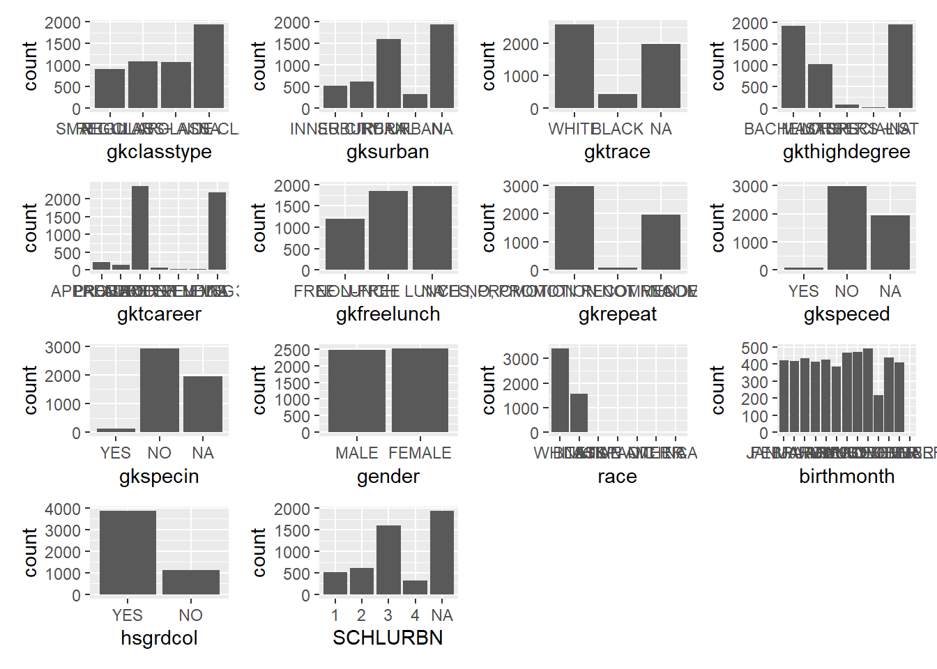 Some of the labels are hard to read. We won’t bother tidying them up, because we merely want to get a feel for the distribution of traits. There is nothing too striking going on. Let’s do something more interesting with numeric variables by splitting them out by graduation success.
star_stud_pl <- star_stud %>%
select(-birthyear) %>%
pivot_longer(where(is.numeric), names_to = "preds", values_to = "value")
ggplot(star_stud_pl, aes(y=value, color=hsgrdcol, fill=hsgrdcol)) +
geom_boxplot(alpha=0.4) +
facet_wrap(~ preds, scales = "free_y") +
theme_minimal()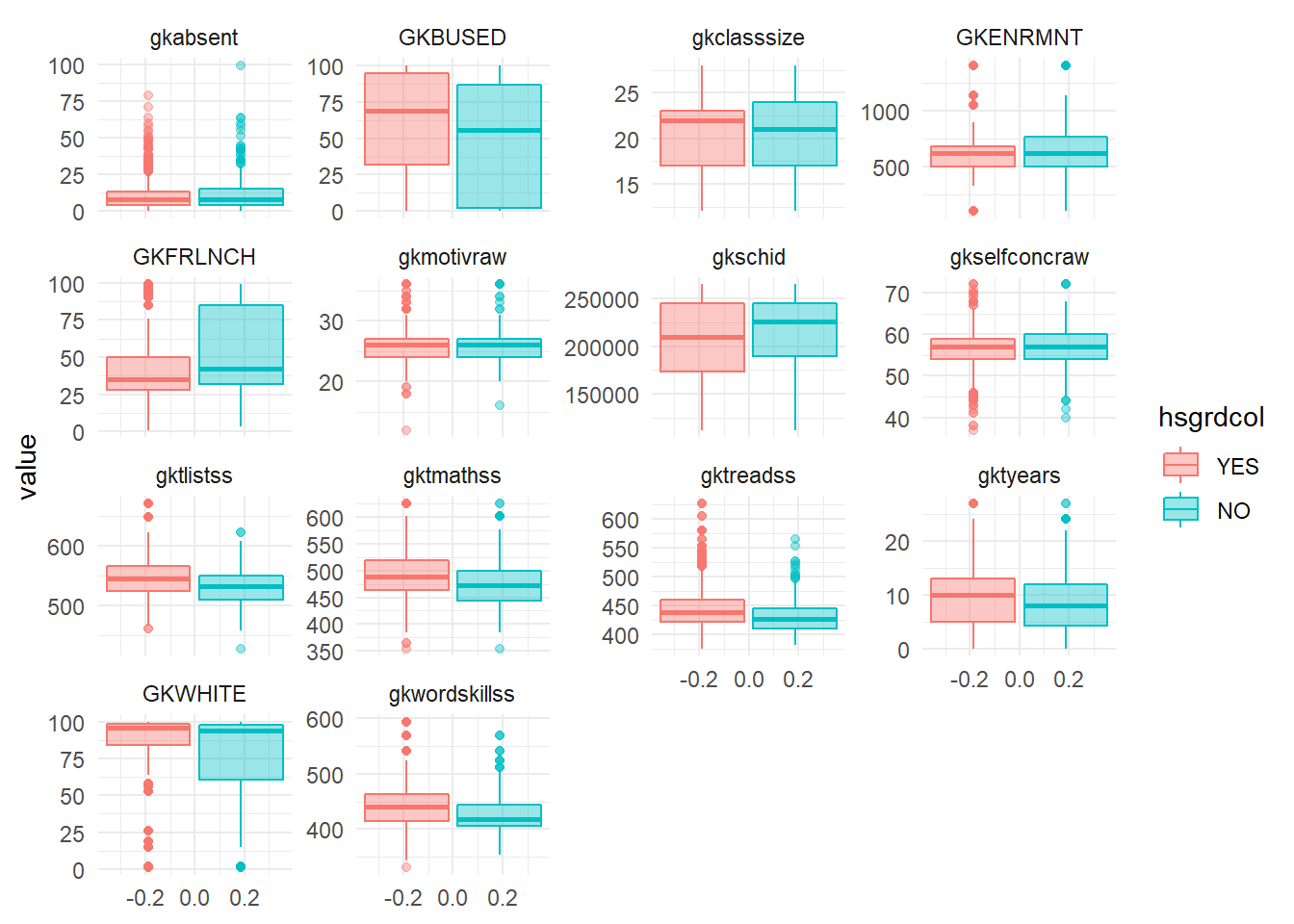 Absenteeism in kindergarten seems a little higher for drop outs, while their skills at reading, listing and math seem lower. Drop outs also more often receive free lunches.
Next, we split the data into a training and test set. In order to make the best use of the training data we have, we then sample from the training data to create five different training data sets. Hopefully, these allow us to build a model that is more robust than if we only relied on the peculiar composition of the initial training data set.
star_split <- initial_split(star_stud, prop=0.8, strata = hsgrdcol)
star_train <- training(star_split)
star_test <- testing(star_split)

# Create cross validation folds, stratify by hsgrcol to avoid adding another type of imbalance
set.seed(290)
star_folds <- vfold_cv(star_train,
                       v = 5,
                       strata = hsgrdcol)
The Models
Our second step is to set up the models we will use in the analysis. We start out with a logistic model and a basic decision tree, which we then refine. We also define the metrics we want to extract out of our models later.
# Logistic regression
star_logist <- logistic_reg() %>%
  set_engine("glm") %>%
  set_mode("classification")

# A basic decision tree
star_tree <- decision_tree() %>%
  set_engine('rpart') %>%
  set_mode('classification')

# random forest trees
star_forest <- rand_forest(
  mtry = tune(),
  trees = 1000,
  min_n = tune() ) %>%
    set_mode("classification") %>%
    set_engine("ranger")

# Create custom metrics
star_metrics <- metric_set(accuracy, roc_auc, sens, spec)
Because decision trees do most of the work in the analysis, we say a little more about how they are made. This helps us understand what we are doing when we tune hyperparameters and how to interpret so called roc curves later on.
In a decision tree, you split the outcome values into two boxes based on one of your predictors. You then split the outcome values in each of the boxes based on another predictor. And so on. So the first split in our case could be between those who have free lunch and those who do not have a free lunch at school.
The algorithm must make two decision at each cut. Which predictor to pick and at which point to make a cut? The solution is not very elegant. Unless variables are continuous, the algorithm simply tries every possible cut for each predictor. It then assign a value to each of the (n dimensions times k predictors) cuts that measures how ‘pure’ the boxes are. You want data points to neatly fall in either box, so that each box is pure. This can be measured by impurity functions such as gini or entropy. The engines in this post happen to use gini, which you may know from measurements of inequality. In the case of two classes, it multiplies the proportion of each in a box together. The resulting value has a maximum for proportions of 0.5. This is indeed the worse you can do if your goal is to make boxes pure!
If you put no limitations and this algorithm, it will keep drawing boxes around graduates and drop outs, until there is a box around every outcome measure. This is unfortunate, because we have molded our model too much to the training data. We have overfit. Hence there is bias. If we applied this model to the test data set, we would probably get very poor predictions.
Putting breaks on the splitting process is a type of so called regularization. It can be done in several ways, such as limiting the number of leafs of the tree, limiting tree depth or setting a minimal size for the nodes (the final subsets). The defaults for these hyperparameters (hyper because they control the splitting criteria, which are the parameters) depend on the package. In the rpart engine for example, the maximum tree depth is 30 and the minimal number of cases per node is 20. There is also a cost-complexity parameter cp that penalizes splits, so the tree doesn’t grow too wildly.
The result of regularization is that we do not have perfect purity in our terminal nodes or, if you will, ultimate boxes. So how to apply the labels then? Typically, a proportion of over 0.5 of a certain label in a terminal node is converted into labeling all the points in the box with that label. This threshold is not set in stone though. The effect of moving it will later be glanced from the so called ROC curve and its associated data frame.
The popularity of decision trees is due to the high quality of the predictions, which require almost no pre-processing of the data and modest computation time.
A Basic Decision Tree
We are now ready to fit a basic decision tree with default hyperparameters.
fit_tree <- workflow() %>%
  add_formula(hsgrdcol ~ .) %>%
  add_model(star_tree) %>%
  fit_resamples(
    resamples = star_folds,
    metrics = star_metrics,
    control = control_resamples(save_pre = T)
  )

fit_tree %>% collect_metrics()
## # A tibble: 4 x 6
## .metric .estimator mean n std_err .config
## <chr> <chr> <dbl> <int> <dbl> <chr>
## 1 accuracy binary 0.780 5 0.00225 Preprocessor1_Model1
## 2 roc_auc binary 0.638 5 0.0135 Preprocessor1_Model1
## 3 sens binary 0.975 5 0.00356 Preprocessor1_Model1
## 4 spec binary 0.104 5 0.0122 Preprocessor1_Model1In the resulting table, we see the mean of the five folds of each of the metrics that we defined earlier. The accuracy is the proportion of predictions that are correct. You may think this is all we would care about, but that is not the case. The third and fourth row contain the metrics that tell you why.
Sens stands for sensitivity, which is the proportion of true YES cases (graduations) we correctly labeled as YES. We got almost all of them. However, the spec stands for specificity, which is the proportion of true NO cases (drop outs) we correctly predicted. Here we got about 10% correct, which is a very low number indeed. A so called confusion matrix gives a picture of what this means in absolute terms.
fit_tree %>%  collect_predictions() %>%
  conf_mat(truth = hsgrdcol,
         estimate = .pred_class)
## Truth
## Prediction YES NO
## YES 3020 803
## NO 77 93If you stare at this table for a while, you realize that out of the 900 kids that eventually dropped out of high school, we identified only a couple. We also glance that if we predict NO for a kindergarten kid we have a poor chance that we’re right.
All of this is not very encouraging. Before we add bells and whistles to the tree, we have to explain the term roc_auc in the table. This term refers to the area under the curve (auc) of the so called ROC curve. We plot is below.
fit_tree %>%
collect_predictions() %>%
roc_curve(hsgrdcol, .pred_YES) %>%
autoplot()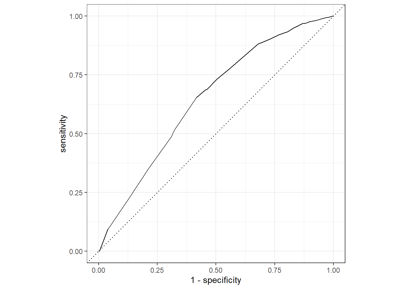 On the y-axis is the sensitivity: the proportion of true graduations that we predicted correctly. On the x-axis is not the specificity, but 1 - the specificity. The word ‘specificity’, recall, refers to the proportion of actual NO’s that we correctly labeled as NO. On the flip side, ‘1 - specificity’ is the remaining proportion of true NO’s that are falsely marked as YES (hence they are called false positives).
It makes sense to plot the proportion of true YES that we caught against false YES labels. For if we labeled everything as YES, out sensitivity would be perfect, but we wouldn’t trust our labels much.
Confusingly, the graph displays all values the sensitivity can take on. So which one belongs to the model? That depends on the threshold for assigning a label to the points in an ultimate node (or box). The standard threshold is 0.5, as we mentioned, but we can set it at whichever value we like. The roc curve displays the sensitivity (and the proportion of false positives) for a whole set of thresholds.
If we set a low threshold for a YES, then we will be less likely to miss a graduation. The cost however is that in that case we cast our net too widely and mistakenly label a lot of drop outs as graduates.
The worst place to be in the graph is the bottom right, where all your predictions are wrong. In the top right, your sensitivity is 1 so that all true YES values are accurately predicted. However, the false positives are also 1, so that all true NO’s are marked as YES. The top left is the best place to be. Every YES and NO is correctly predicted. We can imagine a line going straight up the y-axis and horizontally to the top right of the graph. Below that line the area under the roc curve would be 1 in this ideal case.
The dashed diagonal line represents what would happen if you labeled cases by chance. If you randomly labeled 25% of cases as YES for example, then your sensitivity is expected to be 0.25, but your false positive proportion would also be 0.25. That is, both YES and NO cases are labeled YES 25% of the time. The area under curve in the case of random guessing is the area under the dashed line, which is 0.5.
By looking at the graph or the roc_auc number in the table, we conclude that we have done a little better than chance. The task ahead then is to improve both the roc_auc number and the specificity.
Decision Trees using Resampled Data
One way to deal with the low specificity of our model would be to change the threshold for labeling the points as YES in a box. If this threshold is lower, then more points are labeled NO, and we probably catch more drop outs in our prediction. However, as the roc curve shows, there is trade off with sensitivity. So what we really want is improve the quality of the prediction and get a better roc_auc score.
We do so by writing a so called tidymodels ‘recipe’ for handling the data before it is shoved into a model. The recipe start with setting up the formula. We then impute modes and medians for missing data, because it is fast. If we had more time, we would impute using techniques such as bagged trees or k nearest neighbors. We moreover use the smote algorithm to upsample kids who dropped out of high school with the help of nearest neighbors. Such kids are quite rare in the initial data set so that it is said that this data set is “imbalanced”. Also, identifying drop outs is what we are really interested in, so it makes sense to give the model more cases to train on. We also do some steps that prove useful for more advanced models and for prediction on the test data set.
# prep the data with a recipe
star_rec <- recipe(hsgrdcol ~ ., data = star_train) %>%
  step_impute_mode(all_nominal_predictors()) %>%
  step_impute_median(all_numeric_predictors()) %>%
  step_zv(all_predictors()) %>% # leaves out variables with only a single value
  step_dummy(all_nominal(), -all_outcomes()) %>%
  step_smote(hsgrdcol) %>%
  step_novel(all_predictors(), -all_numeric()) %>%
  step_unknown(all_predictors(), -all_numeric())
We train the same model on the pre-processed data, while also giving it five samples from the initial data of which it will take the mean.
fit_tree_rec <- workflow() %>%
  add_recipe(star_rec) %>%
  add_model(star_tree) %>%
  fit_resamples(
    resamples = star_folds,
    metrics = star_metrics,
    control = control_resamples(save_pre = T)
  )

fit_tree_rec %>% collect_metrics()
## # A tibble: 4 x 6
## .metric .estimator mean n std_err .config
## <chr> <chr> <dbl> <int> <dbl> <chr>
## 1 accuracy binary 0.710 5 0.0101 Preprocessor1_Model1
## 2 roc_auc binary 0.650 5 0.00618 Preprocessor1_Model1
## 3 sens binary 0.767 5 0.0101 Preprocessor1_Model1
## 4 spec binary 0.515 5 0.0170 Preprocessor1_Model1The roc_auc has increased by quite a bit, while the specificity has risen quite spectacularly. This model would identify about half of the drop outs. Because the sensitivity is lower and most kids graduate, we also have a lot more false negatives. Let’s look at the absolute numbers again.
fit_tree_rec %>%  collect_predictions() %>%
  conf_mat(truth = hsgrdcol,
         estimate = .pred_class)
## Truth
## Prediction YES NO
## YES 2374 435
## NO 723 461This time about 2/3 of our predictions of drop outs are wrong. That is still a lot.
Let’s also check how well this decision model does on the test data, that is has not seen before.
tree_wfl <- workflow() %>%
  add_recipe(star_rec) %>%
  add_model(star_tree)

final_res_tree <- last_fit(tree_wfl,
                          star_split,
           metrics = star_metrics)

final_res_tree %>% collect_metrics()
## # A tibble: 4 x 4
## .metric .estimator .estimate .config
## <chr> <chr> <dbl> <chr>
## 1 accuracy binary 0.702 Preprocessor1_Model1
## 2 sens binary 0.799 Preprocessor1_Model1
## 3 spec binary 0.366 Preprocessor1_Model1
## 4 roc_auc binary 0.618 Preprocessor1_Model1We observe that the numbers are very similar, so we haven’t overfit.
The Logistic Model
Before we fit fancier decision trees, we fit a logistic model for reference. We make a workflow object to save a little bit of time as we go along.
# Set up the workflow
star_wkflw <- workflow() %>%
  add_recipe(star_rec)

# fir the logistic model on the folds
logist_f <- star_wkflw %>%
  add_model(star_logist) %>%
  fit_resamples(
    resamples = star_folds,
    metrics = star_metrics,
    control = control_resamples(save_pre = T)
  )

collect_metrics(logist_f)
## # A tibble: 4 x 6
## .metric .estimator mean n std_err .config
## <chr> <chr> <dbl> <int> <dbl> <chr>
## 1 accuracy binary 0.667 5 0.00546 Preprocessor1_Model1
## 2 roc_auc binary 0.720 5 0.00858 Preprocessor1_Model1
## 3 sens binary 0.669 5 0.00647 Preprocessor1_Model1
## 4 spec binary 0.658 5 0.0119 Preprocessor1_Model1We note that accuracy is lower than in the decision trees, but that the roc_auc and relatedly the specificity is higher. We plot the roc curve, this time for each of the five folds, to see if they make a difference.
logist_f %>%
collect_predictions() %>%
group_by(id) %>%
roc_curve(hsgrdcol, .pred_YES) %>%
autoplot()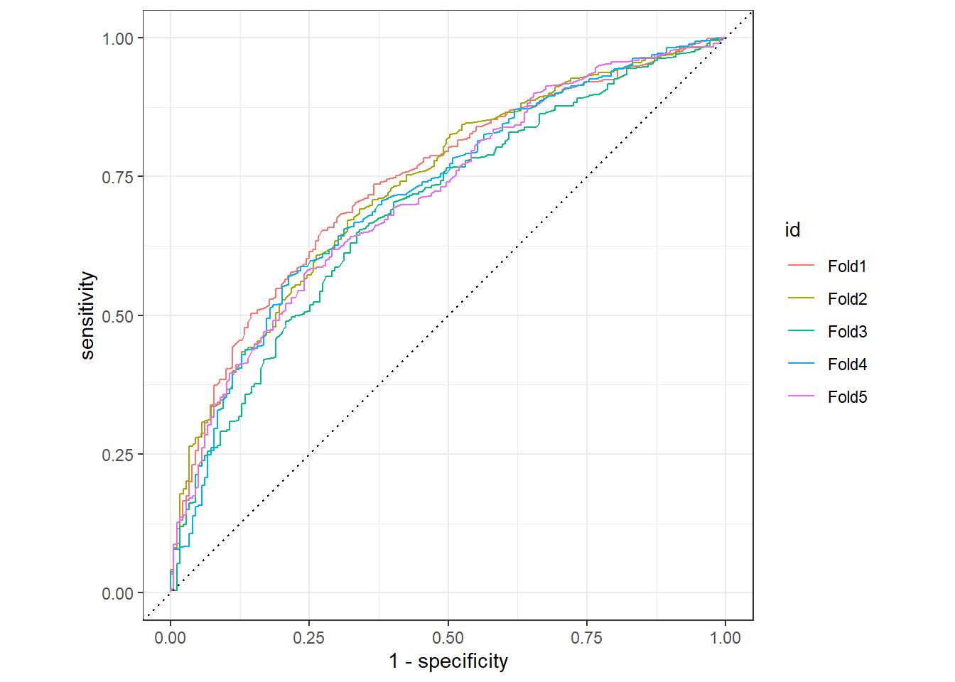 The folds matter quite a bit, so averaging out over them may reduce overfitting.
logist_f %>%
  collect_predictions() %>%
  conf_mat(hsgrdcol, .pred_class)
## Truth
## Prediction YES NO
## YES 2072 306
## NO 1025 590We have labeled yet more drop outs correctly, but still about 2/3 of our NO labels are actually a YES (these are the false negatives). This model doesn’t look so bad. It is to be seen of decision trees can beat it.
To get a rough idea of which predictors make a difference, we check out the results of the logistic model. This idea is rough, because we did not take multicollinearity into account.
log_fit <- star_wkflw %>% add_model(star_logist) %>%
  fit(star_train)

tidy(log_fit, exponentiate=T) %>% filter(p.value <0.05) %>%
  arrange(desc(estimate))
## # A tibble: 19 x 5
## term estimate std.error statistic p.value
## <chr> <dbl> <dbl> <dbl> <dbl>
## 1 race_BLACK 1.85 0.0738 8.34 7.51e-17
## 2 gksurban_RURAL 1.80 0.242 2.44 1.47e- 2
## 3 gkclasstype_REGULAR.CLASS 1.53 0.177 2.40 1.62e- 2
## 4 gkmotivraw 1.10 0.0297 3.09 2.03e- 3
## 5 gkabsent 1.03 0.00468 5.44 5.41e- 8
## 6 gktmathss 0.995 0.00145 -3.34 8.27e- 4
## 7 gktlistss 0.994 0.00186 -3.31 9.46e- 4
## 8 gkwordskillss 0.992 0.00287 -2.69 7.22e- 3
## 9 GKBUSED 0.991 0.00204 -4.67 2.97e- 6
## 10 gkselfconcraw 0.961 0.0146 -2.72 6.46e- 3
## 11 birthmonth_JUNE 0.745 0.148 -1.98 4.74e- 2
## 12 gktrace_BLACK 0.708 0.137 -2.52 1.18e- 2
## 13 gkspecin_NO 0.628 0.209 -2.22 2.62e- 2
## 14 gender_FEMALE 0.595 0.0595 -8.71 2.94e-18
## 15 birthmonth_SEPTEMBER 0.577 0.140 -3.94 8.24e- 5
## 16 birthmonth_NOVEMBER 0.469 0.153 -4.96 7.22e- 7
## 17 birthmonth_DECEMBER 0.366 0.158 -6.36 2.06e-10
## 18 gkfreelunch_NON.FREE.LUNCH 0.358 0.0921 -11.1 7.96e-29
## 19 birthyear 0.331 0.0706 -15.7 3.17e-55Not being in special education seems to greatly improve your chances of graduating, as does being in a rural community and being black. The benefit of the logistic model is that we know how to interpret it. That will turn out to be a little harder for our decision trees.
Let’s see how the logistic model does on the test data set it has not seen before.
logist_wfl <- star_wkflw %>% add_model(star_logist)

final_res_log <- last_fit(logist_wfl,
                          star_split,
           metrics = star_metrics)

final_res_log %>% collect_metrics()
## # A tibble: 4 x 4
## .metric .estimator .estimate .config
## <chr> <chr> <dbl> <chr>
## 1 accuracy binary 0.659 Preprocessor1_Model1
## 2 sens binary 0.672 Preprocessor1_Model1
## 3 spec binary 0.612 Preprocessor1_Model1
## 4 roc_auc binary 0.700 Preprocessor1_Model1The results are very similar to those on the training data, which is as expected. The logistic model draws only one hypersurface through the space of the predictors and the outcome and so is unlikely to overfit.
The logistic model performs strong against basic decision trees. It remains to be seen if fancier trees can beat it, which is discussed in part 2.
Edi Terlaak
I like to tell stories about statistics.