Fundamentals 1: Maximum Likelihood

Theories of Inference

The fundamental puzzle of inference is to say something about an unknown process that generates data, when all you have in your hand are a few of its crumbs. Of course, if you truly understood every aspect of a process, you wouldn’t need to do inference. But especially in the social sciences, this is never the case. So the problem of inference is to put probabilities on outcomes of a process that you do not understand. Although second best, it still gives some grip on reality.

It is hard to make progress with this puzzle unless we make some assumptions. You can do without these assumptions, but that is a topic for another time. To make our life easier, we first assume that the data were independently drawn from a population. Second, we assume that data are generated on the basis of a parametric probability distribution. Think of the Normal, Bernoulli or Poisson distributions. The benefit of these things is that you don’t have to estimate the probability for every possible value of the data. One or two parameters describe the entire probability distribution! Think of the mean and variance for the Gaussian, lambda for the Poisson and p for the Bernoulli. When you are willing to make this assumption, you are doing parametric statistics.

Instead of figuring out probabilities for the values of the process directly then, we estimate one or more parameters that we will call ‘theta’ (\(\theta\)) (theta can be a vector) that control a distribution that indirectly gives us the probabilities for values of the process. So the problem is now transformed from estimating maybe thousands of values into estimating only one or more parameters, based on data and your assumption about a model (say, a linear model with a Gaussian distribution).

We stress the last point here. In inference, the claims about our estimate and its uncertainty are conditional also on the model we picked. Often, we could have chosen a different model just as well. This so called ‘model dependence’ has become a more prominent topic of study in recent years. See for example this article for a case study.

Carrying on, we can now translate the problem of inference into a formula with the help of Bayes’ Rule. Instead of probabilities for events, which typically figure in Bayes’ Rule, we now place probability distributions in the formula. These can be either discrete or continuous. We will not bother with this distinction here.

\[p(\theta|data)=\frac{p(\theta)p(data|\theta)}{p(data)}\] The left hand side of the equation says we want to know the probabilities for values of theta, given the data we have (and the model we picked, but that will be taken for granted going forward). The right hand side gives a formula for calculating it.

Using Bayes’ Rule does not mean we are now doing Bayesian inference! The type of inference depends on the interpretation of the right hand side of the equation. This interpretation in turn depends on your statistical worldview. There are two camps here.

If you are a frequentist, you believe that theta is out there to be discovered. You assume that there is fundamental uncertainty in the world, which can typically be estimated with parametric probability distributions. The parameter theta that controls this distribution is fixed.

If you are a Bayesian, you believe that uncertainty is not fundamental to the world, but a measure of our beliefs in values for the parameters (and thereby in the process that we try to understand). As we learn more, the uncertainty will disappear. Theta is therefore not treated as fixed, but as a random variable. It allows Bayesians to have beliefs about a parameter before seeing the data (based on earlier evidence and scientific theories) and to adjust it based on the data.

Likelihood theory results from the frequentist interpretation of the above formula. Because theta is fixed, \(p(\theta)\) refers to probabilities for values that are not random. These values have either probability 0 or 1. So \(\frac{p(\theta)}{p(data)}\) only depends on the data then - with respect to theta, it is a constant. It is therefore said that the probability of theta is proportional only to the part of the right hand side that is called the likelihood function.

\[p(\theta|data) \propto p(data|\theta)\] This leads to the following definition of likelihood.

\[\cal L(\theta|data) = p(data|\theta)\] Although the math is easier in likelihood, the concept is less intuitive than the Bayesian interpretation, which we will set out in a future post.

Before we go into the details of likelihood inference, we round out our overview by mentioning a third approach to the problem of inference, which is hypothesis testing. It also adheres to the frequentist interpretation, but is not concerned with estimating theta, but rather with testing whether it is different from some value. This may seem like a curious approach to doing statistics, but it is in fact the dominant approach. Much more on this in future posts also. Let’s list the three approaches in no particular order for the sake of clarity.

1. Maximum Likelihood
2. Hypothesis Testing
3. Bayesian inference

It is probably unproductive to approach statistical problems from either only a frequentist or a Bayesian point of view. Both approaches have pros and cons, which we will discuss when we lay out the Bayesian framework. We start this series off with likelihood theory, because the frequentist point of view is still dominant.

Maximum Likelihood

We begin with a maximum likelihood calculation for a simple linear model. There are two components to this model. First, there is the systematic part, which predicts the value of the average \(\mu\) for some covariate. Second, we assume that there is noise around this estimate due to fundamental uncertainty in nature. This is the stochastic part of the model. Here we assume that the noise is normally distributed.

We now run through the calculation of the ML, plugging in \(\beta\) at the very end in order to get used to the idea of reparameterization. This \(\beta\) could be a vector of covariates that predict the value we are interested in. Here however, to keep things simple, it is just a scalar that holds the value of \(\mu\).

Finding the maximum likelihood means maximizing the probability (or density) of the data, given a parameter. In other words, we run through candidate parameters, and pick the ones that make the data the most likely. So for some candidate mean and standard deviation we set up a normal distribution and calculate the probability (technically the density) of this data point. We do this for all data points and multiply the densities together (we can do this because we assume independence; we can still do likelihood inference without this assumption, but in that case things get a whole lot more complicated).

\[\mathcal{L} (\mu_i,\sigma_{i}|y) = \prod_{i=1}^n f(y_{i}|\mu_i,\sigma_{i}) \] The outcome of this calculation is some crazy number that is very small and doesn’t have any intuitive meaning. It virtue is that it helps us find the \(\mu\) and \(\sigma\) that make the data the most likely.

Next, we take the log of both sides, because it allows us to write the product as a sum. This makes it easier to differentiate later. Also, the crazy small number becomes a negative number that is large in absolute value and easier on the eye.

\[ln(\mathcal{L}(\mu_i,\sigma_{i}|y))=\sum_{i=1}^{n}ln(f(y_{i}|\mu_i,\sigma_{i})) \] Filling in the formula for the normal distribution reveals what model we were assuming all along.

\[ln(\mathcal{L} (\mu_i,\sigma_{i}|y))=\sum_{i=1}^{n}ln(\frac{1}{\sqrt{2\pi}\sigma}e^{-\frac{(y_{i}-\mu_{i})^2}{2\sigma^2}}) \] Taking the natural log will simplify things considerably. Since we want to get at the maximum likelihood estimate for the mean, we also drop terms that do not depend on \(\mu\).

\[ln(\mathcal{L}(\mu_i|y,\sigma_{i}))\approx \sum_{i=1}^{n}{-\frac{(y_{i}-\mu_{i})^2}{2\sigma^2}}\] Substituting the scalar \(\beta\) for \(\mu\) (another name for the same thing now, later we will put more stuff in \(\beta\)) and taking the partial derivative of this expression with respect to \(\beta\) shows that the mean is the best estimate for \(\beta\).

This is utterly unsurprising. If we assume that data are normally distributed, then the mean of the data is the best candidate for the \(\mu\) in the normal probability distribution formula. In other words, the normal distribution with the sample mean at its center on average assigns the highest probabilities to such sample data.

Although the ML estimate was unimpressive, it does have nice properties which are helpful in more interesting cases. In particular, if there is an unbiased estimator for a problem, then ML will provide it, while also being efficient. Efficiency is a technical term that means that the variance around the unbiased estimator is minimal. And even if there is no unbiased estimator, ML will come up with a good one.

Let us now demonstrate how we can actually calculate the ML for an example in which we fill \(\beta\) with coefficients of a linear model. That is, the average will depend on some predictor on the x-axis now. The normally distributed noise term is spread out in the up-down direction and moves from left to right centered at the y-value of the line.

Fake data simulation

Instead of using a real world data set, we generate fake data. This allows us to control the systematic and random components of the data generating process. We will then try to reconstruct this data generating process with ML, based on the noisy y-values and the x’s.

In the code below we construct a linear relationship between two variables. This represents the structural component of the process. We then add normal noise to every value of y - the stochastic component of the process. This generates noisy observations.

# choose a slope and an intercept of the data generating process
a_int <- 3
b_slope <- 2
# generate random x-coordinates from uniform distribution
data_x <- runif(n=100, 0,40)
# find the true y's generated by this process
true_y <- data_x * b_slope + a_int
# generate noisy y's that function as our 'observations' of the dependent variable
data_y <- true_y + rnorm(mean=0, sd=4, n=length(true_y))

# add a column of 1's for estimating the intercept later
X <- cbind(1,data_x)
# create dataframe for plotting with ggplot
fake_data <- as.data.frame(cbind(data_x, data_y))
# plot
ggplot(fake_data, aes(x=data_x, y=data_y)) + 
  geom_point() +
  theme_classic() +
  labs(x="dependent variable",
       y="response variable",
       title="Observations from a fake data generating process")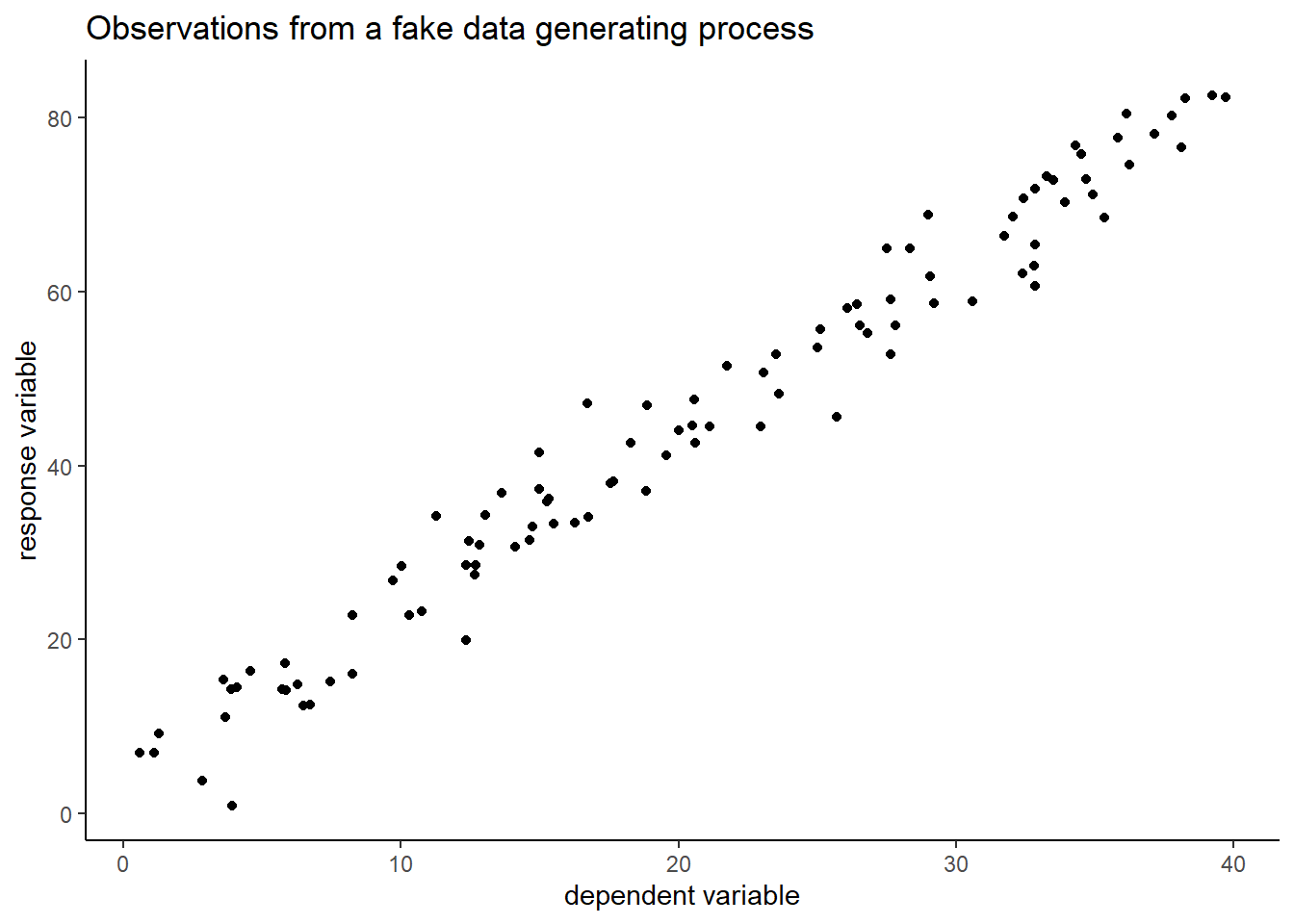

We now code a likelihood function that assumes a linear model for the structural component of the process and a normal distribution for the stochastic component. We then pass this function together with the fake data into the optim function of R, that will find the ML estimates.

# set up a log likelihood function
# theta will contain mu and variance, where mu = a + bX
lf <- function(theta,y,X){
n <- nrow(X)
k <- ncol(X)
# beta will contain estimates for a and b
beta <- theta[1:k]
sigma2 <- theta[k+1]
# pull the error between observed y and estimates outside formula of normal dist
e <- y-X%*%beta
# log of the formula for the normal distribution
logl <- -.5*n*log(2*pi)-.5*n*log(sigma2)-
  ((t(e)%*%e)/(2*sigma2))
# return negative because optim likes to minimize
return(-logl)
}

# pass data and likelihood function to optim; we also pass guessed values, to get optim on to a good start
p<-optim(c(5,2,4),lf,method="BFGS",hessian=T,y=data_y,X=X)
# print out the paramter estimates
p$par

## [1]  4.176248  1.976342 14.897150

Let’s check how well ML has done. It estimates 4.18 for the intercept (true value 3) and 1.98 for the slope (true value 2). The real variance was 16 and is estimated to be 14.9.

We had only 65 data points, so we should give our model some slack. How much slack? That can also be computed from the likelihood formula in the form of standard errors. What follows is a bit of a technical story, but it hopefully gives some intuition for where standard errors come from.

We start by taking second partial derivatives of the log-likelihood function with respect to the paramaters. We can arrange these values in a matrix. We do this in such a way that we get a so called Hessian matrix. \[\mathbf{H}(\theta)=\frac{\partial^{2}}{\partial\theta_{i}\partial\theta_{j}}ln(\mathcal{L}(\theta))\] You may remember this matrix from a calculus class where you approximated some wild surface with a quadratic graph. In the process, you had to calculate the Hessian. This is what we are doing for wild likelihood surfaces (not the ones we are dealing with in this post) as well. We approximate them with a quadratic surface. If you evaluate the Hessian at a critical point (here: the maximum of the likelihood surface), it gives you information about the curvature. What matters here is that it tells you the steepness near the peak. If the region around the peak is very steep, then you are more certain of your estimate.

If you multiply the Hessian by -1 you get a matrix that is called the observed Fisher Information (I). You do this because the second derivative at a maximum is negative. So this operation cancels that minus sign and makes the Fisher Information positive. \[\mathbf{I}(\theta)=-\frac{\partial^{2}}{\partial\theta_{i}\partial\theta_{j}}ln(\mathcal{L}(\theta))\] So a bigger value for I means that the curvature around the maximum is greater. This is a good thing, because it means you are more sure of your estimate.

Next, if we take the inverse of the Fisher Information, we get the variance of the maximum likelihood estimate. \[\mathrm{Var}(\hat{\theta}_{\mathrm{ML}})=[\mathbf{I}(\hat{\theta}_{\mathrm{ML}})]^{-1}\] We skip the derivation, which is actually not too bad. More work is the stronger claim that the ML estimates are normal in distribution as n gets larger. \[\hat{\theta}_{\mathrm{ML}}\stackrel{a}{\sim}\mathcal{N}\left(\theta_{0}, [\mathbf{I}(\hat{\theta}_{\mathrm{ML}})]^{-1}\right)\] A proof can be found here. This result looks like the Central Limit Theorem (CLT), but is more general. After all, \(\hat{\theta}_{\mathrm{ML}}\) does not only stand for the mean (as in the CLT), but can be any parameter that we care about in the model.

We will now approximate this distribution with data from our sample. We already multiplied the output of the lf function by -1 in the code, so we just need to invert the Hessian that optim spits out to get the Fisher Information matrix. If we take the square root of the diagonal entries, we can read off the standard errors of our coefficients. We compare them with the output of lm, which calculates standard errors via another route.

# invert hessian to calculate Fisher Information matrix
OI<-solve(p$hessian)

# standard errors are squared values on diagonal
se <- sqrt(diag(OI))
se

## [1] 0.81242919 0.03480456 2.10817070

# Compare with OLS using lm
dat_fake <- as.data.frame(cbind(X,data_y))
summary(lm(data=dat_fake, data_y ~ 1 + data_x))

## 
## Call:
## lm(formula = data_y ~ 1 + data_x, data = dat_fake)
## 
## Residuals:
##      Min       1Q   Median       3Q      Max 
## -10.9670  -2.0510   0.0539   2.4401   9.9184 
## 
## Coefficients:
##             Estimate Std. Error t value Pr(>|t|)    
## (Intercept)  4.17576    0.82041    5.09 1.73e-06 ***
## data_x       1.97636    0.03515   56.23  < 2e-16 ***
## ---
## Signif. codes:  0 '***' 0.001 '**' 0.01 '*' 0.05 '.' 0.1 ' ' 1
## 
## Residual standard error: 3.898 on 98 degrees of freedom
## Multiple R-squared:  0.9699, Adjusted R-squared:  0.9696 
## F-statistic:  3162 on 1 and 98 DF,  p-value: < 2.2e-16

We note that the estimates of the standard error by optim and lm are practically the same. The standard error of 0.812 around the intercept means that we are not surprised we were off by 1.18.

Simulating From a Likelihood Model

If ML gives the same information as lm, we may wonder why we should bother. One answer is that ML can also be applied when the covariates have a nonlinear relation with the response. Another answer is that we have more freedom in simulating whichever quantity of interest we care about.

We illustrate the point about simulation with a data set that measures math anxiety in Belgian and German primary school teachers. As predictors, we look at the age, gender and experience of teachers. We go through the same steps as in the fake data example so as to come up with estimates and standard errors.

# we select the variables we need and make everything numeric
# We simply drop NAs, because we are not really concerned with precise estimation
DAT <- data %>% mutate(gender = recode(gender,
                                       "f" = 0,
                                       "m" = 1)) %>% 
  select(age, gender, experience_level, math_anxiety) %>% 
  drop_na() %>% 
  mutate_all(as.numeric) %>% 
  as.matrix()

DAT <- cbind(1,DAT)
# y_dat is observed math anxiety
y_dat <- DAT[,5]
# x_dat are predictors
x_dat <- DAT[,1:4]

# using the same lf function defined earlier we optimize
est_teach <- optim(c(15,0.3,-6,-0.3,20),lf,method="BFGS",hessian=T,y=y_dat,X=x_dat)
# print the parameters
est_teach$par

## [1] 15.4959389  0.2626861 -6.5682221 -0.3104229 50.6004609

# create Fisher information matrix
FI <-solve(est_teach$hessian)

This time around, we want to simulate from these estimates. We can do so in two ways.

A first option is to generate predictions. If we for example want to estimate the math anxiety of a female teacher of average age and a median level of experience, then we have to take into account both estimation uncertainty (the standard error around our coefficient estimates) as well as fundamental uncertainty (the normally distributed noise, estimated by sigma).

Below, we first take 1000 draws from the multivariate normal with mean our ML estimates and variance the Fisher information matrix. We then create a vector of the values of the covariates that belong to the individuals we care about.

# sample from multivariate normal, with mean the ML estimates and variance-covariance matrix FI
sim_betas <- rmvnorm(n=1000, mean=est_teach$par, FI)

# prediction for female teacher of average age and median experience
pred <- as.numeric(c(1, mean(data$age), 0, median(data$experience_level, na.rm=T),0 ) )

set.seed(123)
# now simulate, adding fundamental uncertainty to estimation uncertainty
sim <- as.data.frame(apply(sim_betas, 1, function(x) {
  rnorm( 1, mean=pred%*%x, sd=sqrt(est_teach$par[5]) )} ) )
# create a simple plot
a <- mean(sim[,1])
ggplot(sim, aes(x=sim[,1])) + 
  geom_density() +
  geom_vline(xintercept =a, linetype="dotted", 
             color = "red", size=1, label="test") +
  theme_classic() +
  labs(title="Predicted Math Anxiety of Primary School Teachers",
       x="Math Anxiety") +
  geom_text(aes(x = a + 3, y = 0.01, label = "mean"), color="red") +
  xlim(-15,45)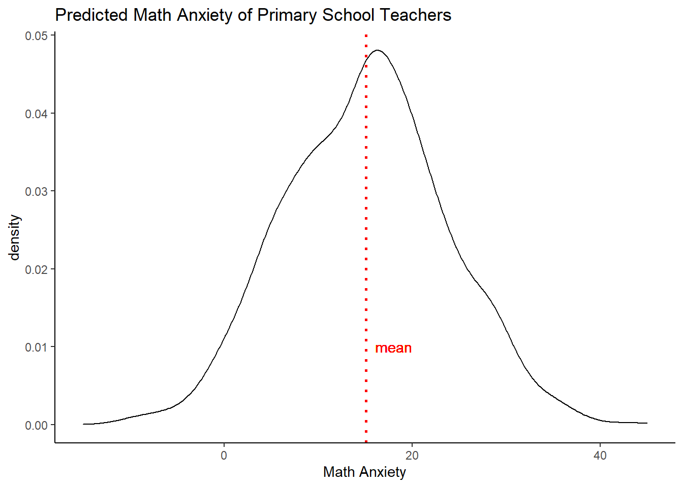

We see the uncertainty spread out before us.

But maybe we want to know what the math anxiety on average will be for the same type of teacher. We can do that too, by averaging over both types of uncertainty, so that the fundamental uncertainty should cancel out.

set.seed(02138)
# repeat, but now take the means of simulating over both types of uncertainty a thousand times
expectedsim <- as.data.frame(apply( sim_betas, 1, function(x) {
  mean(rnorm( 1000, mean=pred%*%x, sd=sqrt(est_teach$par[5])) )} ) )

# create a simple plot
a <- mean(expectedsim[,1])
ggplot(expectedsim, aes(x=expectedsim[,1])) + 
  geom_density() +
  geom_vline(xintercept =a, linetype="dotted", 
             color = "red", size=1, label="test") +
  theme_classic() +
  labs(title="Expected Value Math Anxiety of Primary School Teachers",
       x="Math Anxiety") +
  geom_text(aes(x = a + 3, y = 0.01, label = "mean"), color="red") +
  xlim(-15,45)

## Warning: Ignoring unknown parameters: label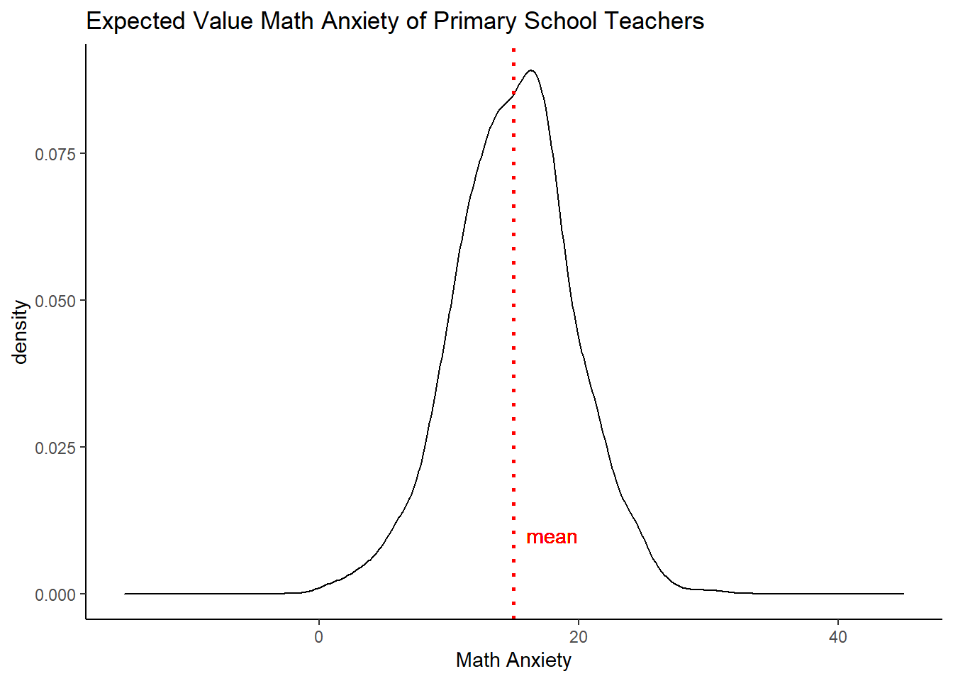

As expected, the uncertainty has been reduced, but based on these data, we are not even that confident saying what the average math anxiety will be for this group of teachers. The estimation uncertainty alone prevents this.