Math, Grit and Machine Learning
In previous posts on the Grit study we saw that it was difficult to estimate the effect of the grit intervention on math scores, even though we have data from a large experiment involving thousands of children. The reason was that the assignment to the intervention and control groups was not randomized at the level of the individual but at the level of the school.
In this post we attempt to balance properties of kids in the study evenly across the groups with the help of BART, short for Bayesian Additive Regression Trees. These regression trees are a machine learning method in which explanatory variables (aka covariates) are cut at certain points so that values below the value are assigned one estimate of y (what we want to explain) and values above another. After a given number of cuts are made the process stops. The resulting estimate of y is subtracted from the actual value of y and the process is repeated for the residuals. In this way, many trees are built, so that there is a risk of overfitting: fitting the model to the sample data and not to the underlying data generating process.
In so called boosting algorithms, this problem is solved by limiting the depth of the trees (that is, the number of branching points per tree) and multiplying all trees by a small number, so that the impact of a tree that models twists and turn in the data and not the data generating process is limited. In BART, this problem is solved by setting priors for both the tree depth and the multiplier. In this way, if the signal is strong, the data can override the regularization we put on the model to prevent it from fitting noise.
We load the required packages and the data. This time we also load data from sample 1, which did not properly assign children to the control and intervention groups. We can now include this data however, because the flexible BART model allows us to control for confounders. The BART model is very good at these kinds of causal estimations, since it was one of the winners of a 2016 causal prediction tournament.
library(bartCause)
library(tidyverse)
library(haven)
library(janitor)

# load data from the two samples
sample1 <- read_dta("Sample1_Data.dta")
sample2 <- read_dta("Sample2_Data.dta")

# compare the columns of the two data sets
compare_df_cols(sample1, sample2, return="match")
## column_name sample1 sample2
## 1 age numeric numeric
## 2 alldiff numeric numeric
## 3 avpayoffv1 numeric numeric
## 4 belief_survey1 numeric numeric
## 5 belief_survey2 numeric numeric
## 6 bothpayoffs numeric numeric
## 7 choicer1 numeric numeric
## 8 choicer2 numeric numeric
## 9 choicer3 numeric numeric
## 10 choicer4 numeric numeric
## 11 choicer5 numeric numeric
## 12 choicev2 numeric numeric
## 13 classid numeric numeric
## 14 confidence_survey2 numeric numeric
## 15 csize numeric numeric
## 16 difficult_imposedr1 numeric numeric
## 17 difficult_imposedv2 numeric numeric
## 18 grit numeric numeric
## 19 grit_survey1 numeric numeric
## 20 grit_survey2 numeric numeric
## 21 inconsistent numeric numeric
## 22 male numeric numeric
## 23 mathgrade2 numeric numeric
## 24 mathscore1 numeric numeric
## 25 mathscore2 numeric numeric
## 26 mathscore3 <NA> numeric
## 27 patience numeric <NA>
## 28 payoffr1 numeric numeric
## 29 payoffr2 numeric numeric
## 30 payoffr3 numeric numeric
## 31 payoffr4 numeric numeric
## 32 payoffr5 numeric numeric
## 33 payoffv2 numeric numeric
## 34 playedr1 numeric numeric
## 35 playedv2 numeric numeric
## 36 raven numeric numeric
## 37 risk numeric numeric
## 38 sample numeric numeric
## 39 schoolid numeric numeric
## 40 studentid numeric numeric
## 41 success numeric numeric
## 42 successr1 numeric numeric
## 43 successr2 numeric numeric
## 44 successr3 numeric numeric
## 45 successr4 numeric numeric
## 46 successr5 numeric numeric
## 47 successv2 numeric numeric
## 48 task_ability numeric numeric
## 49 verbalgrade2 numeric numeric
## 50 verbalscore1 numeric numeric
## 51 verbalscore2 numeric numeric
## 52 verbalscore3 <NA> numeric
## 53 wealth numeric numeric# combine data sets and remove columns that appear in only one of them
sample_comb <- bind_rows(sample1,sample2) %>%
select(-c(mathscore3, patience,verbalscore3))We furthermore use only those rows that contain no missing values. (Given more time we would impute missing values.) Unfortunately, BART cannot solve the problem of selecting variables that are relevant. We therefore first run the BART model on sample 2 with the variables specified by the researchers, as we did in the previous blog post.
Unlike regular machine learning trees, BART can estimate the effect of the intervention variable and calculate the uncertainty.
# drop rows with NA values
sample2_drop <- drop_na(sample2)

# select the independent vars from original study
data_explan <- sample2_drop %>%
  select(male,raven,csize, belief_survey1,mathscore1) %>%
  as.matrix()

# select dependent variable
data_dep <- sample2_drop %>%
  select(mathscore2) %>%
  as.matrix()

# select grit, which is the treatment variable
treatment <- sample2_drop %>%
  select(grit) %>%
  as.matrix()

bartc1 <- bartc(data_dep, treatment, data_explan,
                method.rsp = "bart",
                method.trt = "bart",
                estimand = "ate",
                group.by = NULL,
                commonSup.rule = "none",
                commonSup.cut = c(NA_real_, 1, 0.05),
                args.rsp = list(), args.trt = list(),
                p.scoreAsCovariate = FALSE, use.ranef = TRUE, group.effects = FALSE,
                crossvalidate = FALSE,
                keepCall = TRUE, verbose = TRUE)
## fitting treatment model via method 'bart'
## fitting response model via method 'bart'summary(bartc1)## Call: bartc(response = data_dep, treatment = treatment, confounders = data_explan,
## method.rsp = "bart", method.trt = "bart", estimand = "ate",
## group.by = NULL, commonSup.rule = "none", commonSup.cut = c(NA_real_,
## 1, 0.05), args.rsp = list(), args.trt = list(), p.scoreAsCovariate = FALSE,
## use.ranef = TRUE, group.effects = FALSE, crossvalidate = FALSE,
## keepCall = TRUE, verbose = TRUE)
##
## Causal inference model fit by:
## model.rsp: bart
## model.trt: bart
##
## Treatment effect (pate):
## estimate sd ci.lower ci.upper
## ate 0.1591 0.1175 -0.07113 0.3893
## Estimates fit from 353 total observations
## 95% credible interval calculated by: normal approximation
## population TE approximated by: posterior predictive distribution
## Result based on 500 posterior samples times 10 chainsWe note an estimated effect of grit of only 0.16 with a meaty uncertainty. Unlike the standard error in classical regression, the sd of the posterior does not necessarily describe a normal distribution. It make sense, therefore, to plot it.
plot_indiv(bartc1)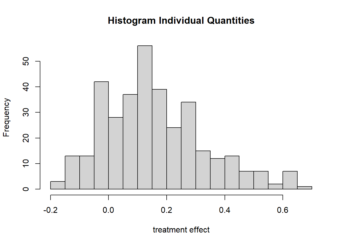
We observe that there is probably a treatment effect, but that it is probably smaller than both in the original author’s study and our multilevel model with imputed values.
We can hope to reduce the uncertainty in our estimation by including more observations. We therefore add the observations from the first sample and run the same model.
# remove NA_s
sample_comb_no_NA <- sample_comb %>%
drop_na()

data_explan <- sample_comb_no_NA %>%
  select(male,raven,csize, belief_survey1,mathscore1) %>%
  as.matrix()

# select mathscore2, which is the math performance after the intervention
data_dep <- sample_comb_no_NA %>%
  select(mathscore2) %>%
  as.matrix()

# select grit, which is the treatment variable
treatment <- sample_comb_no_NA %>%
  select(grit) %>%
  as.matrix()

bartc2 <- bartc(data_dep, treatment, data_explan,
                method.rsp = "bart",
                method.trt = "bart",
                estimand = "ate",
                group.by = NULL,
                commonSup.rule = "none",
                commonSup.cut = c(NA_real_, 1, 0.05),
                args.rsp = list(), args.trt = list(),
                p.scoreAsCovariate = FALSE, use.ranef = TRUE, group.effects = FALSE,
                crossvalidate = FALSE,
                keepCall = TRUE, verbose = TRUE)
## fitting treatment model via method 'bart'
## fitting response model via method 'bart'summary(bartc2)## Call: bartc(response = data_dep, treatment = treatment, confounders = data_explan,
## method.rsp = "bart", method.trt = "bart", estimand = "ate",
## group.by = NULL, commonSup.rule = "none", commonSup.cut = c(NA_real_,
## 1, 0.05), args.rsp = list(), args.trt = list(), p.scoreAsCovariate = FALSE,
## use.ranef = TRUE, group.effects = FALSE, crossvalidate = FALSE,
## keepCall = TRUE, verbose = TRUE)
##
## Causal inference model fit by:
## model.rsp: bart
## model.trt: bart
##
## Treatment effect (pate):
## estimate sd ci.lower ci.upper
## ate 0.2472 0.06801 0.1139 0.3805
## Estimates fit from 1052 total observations
## 95% credible interval calculated by: normal approximation
## population TE approximated by: posterior predictive distribution
## Result based on 500 posterior samples times 10 chainsAdding more observations has not only reduced uncertainty, but increased the estimated effect of the grit intervention to 0.25.
plot_indiv(bartc2)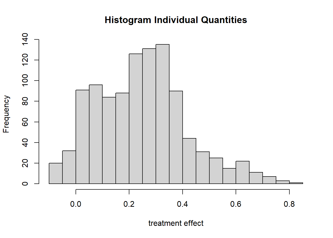
Even though there are samples from the posterior around zero, most are centered around 0.3, which is close to the original estimate of the authors based on sample 2.
Again, we note here the instability of the model given variable selection. Wealth is not perfectly balanced between the control and intervention groups for the combined data set of sample 1 and 2 either.
library(forcats)

# re_name grit
sample_comb <- sample_comb %>% mutate(grit = as_factor(grit),
                                      grit = fct_recode(grit,
                                                           "control" = "0",
                                                           "intervention" = "1"
                                      ))

# distribution of wealth between control and intervention groups
sample_comb %>% ggplot(aes(x=wealth, fill = grit)) +
  geom_bar(aes(y=..prop..), position="dodge") +
  scale_fill_manual(values=c("#157EC9", "#FF6644")) +
  ylab("proportion") +
  theme_classic()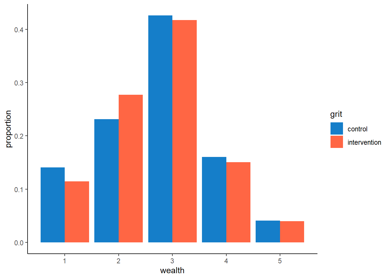
A case could also be made that the school and class effects as well as wealth must be taken into account. So let’s add them to the BART model.
# add more explanatory variables
data_explan_vars <- sample_comb_no_NA %>%
  select(male,raven,csize, belief_survey1,mathscore1, wealth, age, schoolid, classid) %>%
  as.matrix()


bartc4 <- bartc(data_dep, treatment, data_explan_vars,
                method.rsp = "bart",
                method.trt = "bart",
                estimand = "ate",
                group.by = NULL,
                commonSup.rule = "none",
                commonSup.cut = c(NA_real_, 1, 0.05),
                args.rsp = list(), args.trt = list(),
                p.scoreAsCovariate = FALSE, use.ranef = TRUE, group.effects = FALSE,
                crossvalidate = FALSE,
                keepCall = TRUE, verbose = TRUE)
## fitting treatment model via method 'bart'
## fitting response model via method 'bart'summary(bartc4)## Call: bartc(response = data_dep, treatment = treatment, confounders = data_explan_vars,
## method.rsp = "bart", method.trt = "bart", estimand = "ate",
## group.by = NULL, commonSup.rule = "none", commonSup.cut = c(NA_real_,
## 1, 0.05), args.rsp = list(), args.trt = list(), p.scoreAsCovariate = FALSE,
## use.ranef = TRUE, group.effects = FALSE, crossvalidate = FALSE,
## keepCall = TRUE, verbose = TRUE)
##
## Causal inference model fit by:
## model.rsp: bart
## model.trt: bart
##
## Treatment effect (pate):
## estimate sd ci.lower ci.upper
## ate 0.1581 0.09501 -0.02809 0.3443
## Estimates fit from 1052 total observations
## 95% credible interval calculated by: normal approximation
## population TE approximated by: posterior predictive distribution
## Result based on 500 posterior samples times 10 chainsThe estimate now drops again to about 0.14.
Finally, we return to the author’s variable selection and try to enhance our estimation of the causal impact of grit by excluding children who have extreme values for certain properties. For example, if a child in the intervention group would have an extremely high IQ, we may not be able to find a counterpart in the control group. Consequently, we cannot estimate what would have happened in an alternative universe where the high IQ child would not have undergone the grit training program. So we exclude an individual if there is no counterpart within half a standard deviation of the spread of a property.
# Repeat with common support set to "sd" is 1
bartc3.1 <- bartc(data_dep, treatment, data_explan,
                method.rsp = "bart",
                method.trt = "bart",
                estimand = "ate",
                group.by = NULL,
                commonSup.rule = "sd",
                commonSup.cut = 0.5,
                args.rsp = list(), args.trt = list(),
                p.scoreAsCovariate = FALSE, use.ranef = TRUE, group.effects = FALSE,
                crossvalidate = FALSE,
                keepCall = TRUE, verbose = TRUE)
## fitting treatment model via method 'bart'
## fitting response model via method 'bart'# Plot shows which observations are dropped
plot_support(bartc3.1)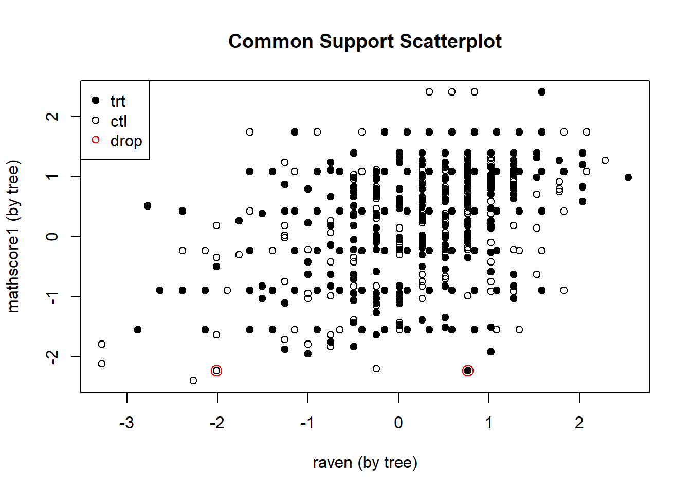
We notice that only one two observation are dropped because they do not have a counterpart.
summary(bartc3.1)## Call: bartc(response = data_dep, treatment = treatment, confounders = data_explan,
## method.rsp = "bart", method.trt = "bart", estimand = "ate",
## group.by = NULL, commonSup.rule = "sd", commonSup.cut = 0.5,
## args.rsp = list(), args.trt = list(), p.scoreAsCovariate = FALSE,
## use.ranef = TRUE, group.effects = FALSE, crossvalidate = FALSE,
## keepCall = TRUE, verbose = TRUE)
##
## Causal inference model fit by:
## model.rsp: bart
## model.trt: bart
##
## Treatment effect (pate):
## estimate sd ci.lower ci.upper
## ate 0.2431 0.06806 0.1097 0.3765
## Estimates fit from 1050 total observations
## 95% credible interval calculated by: normal approximation
## population TE approximated by: posterior predictive distribution
##
## Common support enforced by cutting using 'sd' rule, cutoff: 0.5
## Suppressed observations:
## trt ctl
## 1 1
##
## Result based on 500 posterior samples times 10 chainsThe estimated effect has decreased slightly as a result. It would seem then that there probably is an effect of the grit intervention on math scores if we believe in the variable selection of the authors.
Edi Terlaak
I like to tell stories about statistics.