How big is the testing effect?

Last updated on Jan 20, 2021 16 min read

Students and teachers are united in their dislike of tests. Students get stressed out by cramming and teachers by grading. According to a growing movement among researchers of education, this sentiment is unfortunate, because they think that taking a test after learning improves the score on a subsequent test. This effect is called the testing effect or the retrieval effect. They therefore aim to disassociate testing from evaluation, and aim to rebrand it as a learning tool.

However, many movements in education reform are well-meaning, but flawed. They are often driven by ideology and supported by pseudo-science, arm-chair speculation or an extremely biased interpretation of the evidence. Movements that come to mind are those that promote the idea that there are learning styles or the idea that all children benefit from discovery-based learning.

So how strong is the evidence for the so called testing effect? In this article we will look at a recent study in Nature that answers this question. We reanalyze the data from a Bayesian point of view. In the process, we not only get an idea about the strength of the evidence for the testing effect, but learn a principled way of how to assess the strength of evidence in general.

The study design

The evidence for the analysis comes from a French study by Alice Latimier and colleagues, that investigated how much people learn from a couple of short texts on biology. The segments were supposed to mimic the treatment of DNA in a high school biology textbook. A lot of research has already been done on the testing effect, and we will discuss that later. What Lamitier wanted to know was what type of testing is more effective: testing yourself before you see a text that you will learn or afterwards.

To this end, she recruited over 300 people to participate in an online experiment that she divided into three groups. All of them learned the texts on DNA and then took a test eight days later. The way they learned differed though.

The first group, called ‘Reading-reading’ simply studied the text two times, for as long as they wanted. Supposedly, what they did was read the text and then somehow memorize the pieces of information. We don’t know what strategies they actually used in their head. This condition is typically referred to as ‘re-reading’, assuming that not much else is going on inside the head of participants. The second group took a quiz about DNA first, and only then read the text segments on DNA. The idea is that the quiz question prime people for relevant information they are about to read, so it is memorized better. The third group read the text first, and then took the quiz.

What do you think is most effective? A plausible case can be made for all three approaches. Fortunately, we do not have to rely on intuition, but can use previous studies to inform what we believe before we see the evidence from the study. We will refer to these beliefs before seeing the data as ‘priors’. They will turn out to play a crucial role in inference.

The data

But back to the data. We learn from the Latimier article that 44 participants did not take the final test, 4 did not even complete the training phase and 1 took the learning phase twice a day. All these cases have been dropped from the publicized data set. Hence it is not possible to correct for these missing data. No mention is made of imputation efforts. We also do not learn from which groups the participants dropped out. Given that more than 10% of observations are missing, this omission could seriously influence the results.

Efforts have been made to reduce measurement error from participants who fill in questions blindly. To this end, nine so called ‘catch’ question have been inserted into the quiz. Let’s look at the percentage of participants that answered them correct.

test %>% ggplot(aes(x=score_perc_Catch_exam)) +
  geom_histogram() +
  theme_classic()

## `stat_bin()` using `bins = 30`. Pick better value with `binwidth`.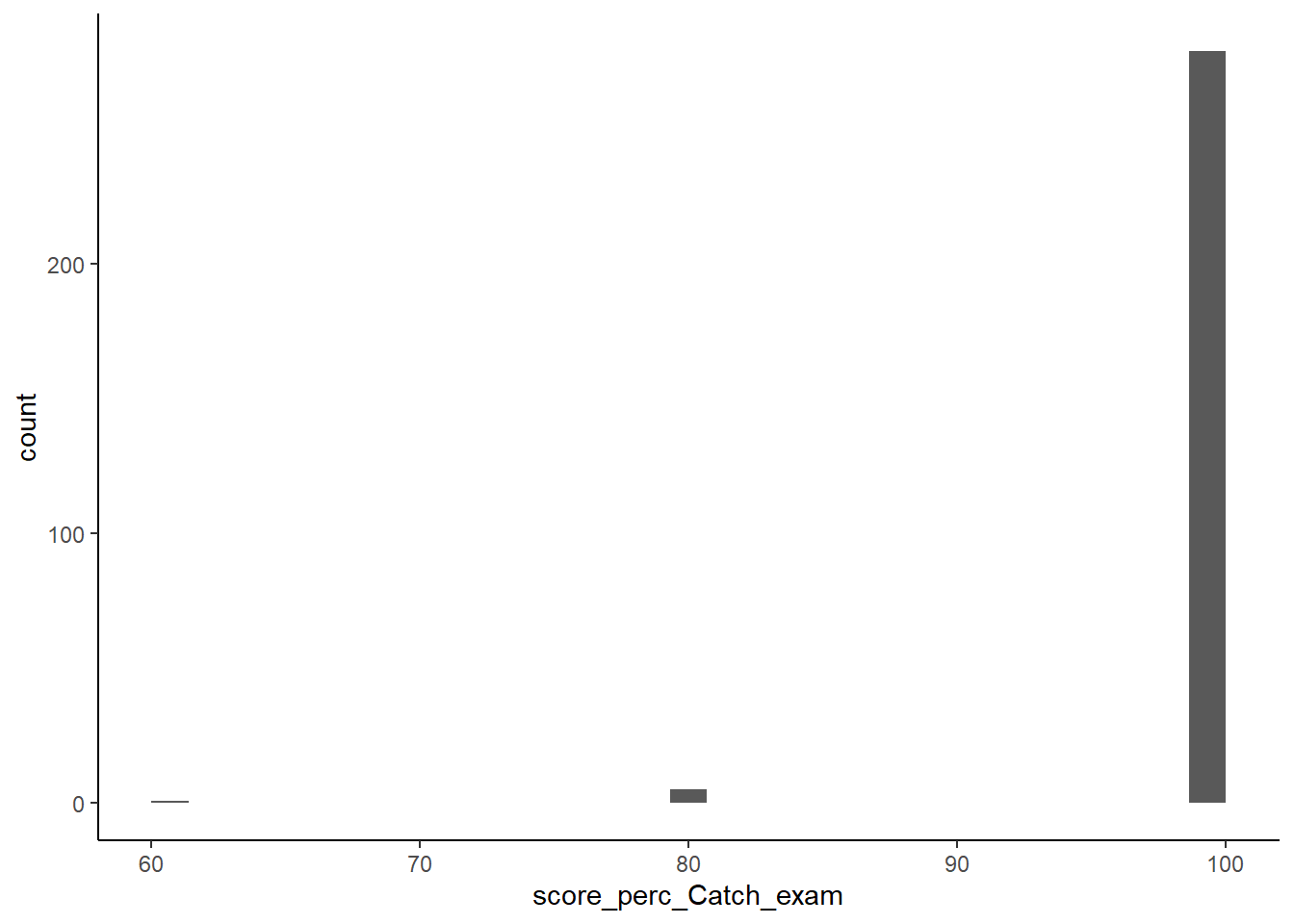

We notice that the catch questions have been answered mostly correct by everyone and see no reason to leave anyone out.

There have been measurements on the time participants spent on the two learning phases, but these have not made it to the public data set. We also do not have access to information on the education level of participants, but this level was equally high in all three groups, so should not interfere with the causal chains. We do have measurements on the types of questions that were on the exam however. These fall into two categories: Trained (same questions as on the quiz) and Untrained (different questions). The latter is subdivided into the categories New (same difficulty level as the quiz questions) and General (knowledge must be transferred to a new situation). This last claim can be verified from the data set.

identical(test$scoreUntrained_exam,(test$scoreNew_exam+test$scoreGeneral_exam))

## [1] TRUE

Exploration of the data

Let us now explore the data visually to see what is going on in the three groups. The benefit of a visual representation is that we learn more than just the position of the mean or median; we also learn the shape of the distribution. We first look at the scores on all the questions per group.

library(patchwork)

test %>% ggplot(aes(x=fct_relevel(learning_condition, "Reading-reading", "Quiz-reading", "Reading-quiz"), y = score_perc_Total_exam)) +
  geom_jitter(width = 0.1, alpha=0.5) +
  labs(y="total score exam",
       x="groep") +
  #coord_flip() +
  theme_classic()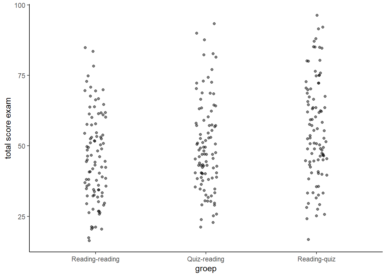

We observe that as we move from re-reading to quizing before seeing the text to quizing after we see the text, the scores tend to go up. We also note that there is no dramatic effect. It is as if every benefits just a little bit.

If we look at the scores on the questions that have been aswered during the training phas (for the last two groups), we notice that the effect is bigger.

p2 <- test %>% ggplot(aes(x=fct_relevel(learning_condition, "Reading-reading", "Quiz-reading", "Reading-quiz"), y = score_perc_Trained_exam)) +
  geom_jitter(width = 0.1, alpha=0.5) +
  labs(y="trained score exam",
       x="groep") +
  #coord_flip() +
  theme_classic()

p3 <- test %>% ggplot(aes(x=fct_relevel(learning_condition, "Reading-reading", "Quiz-reading", "Reading-quiz"), y = score_perc_Untrained_exam, color=scoreNew_exam)) +
  geom_jitter(width = 0.1, alpha=0.5) +
  labs(y="untrained score exam",
       x="groep") +
  #coord_flip() +
  theme_classic()

p2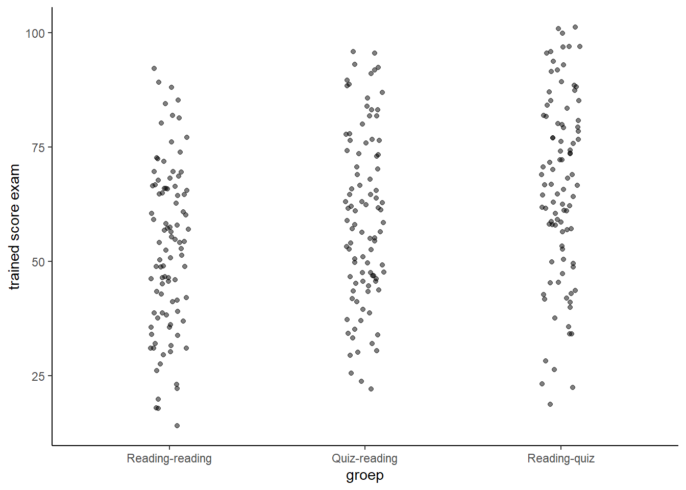

Let us inspect the effect of different types of questions for each group side-by-side.

d1 <- test %>% ggplot(aes(x=score_perc_Total_exam)) +
  geom_density() +
  labs(x="total score exam") +
  facet_wrap(vars(fct_relevel(learning_condition, "Reading-reading", "Quiz-reading", "Reading-quiz")), nrow = 3) +
  #coord_flip() +
  theme_classic()

d2 <- test %>% ggplot(aes(x=score_perc_Untrained_exam)) +
  geom_density() +
  labs(x="untrained score exam") +
  facet_wrap(vars(fct_relevel(learning_condition, "Reading-reading", "Quiz-reading", "Reading-quiz")), nrow = 3) +
  #coord_flip() +
  theme_classic()

d3 <- test %>% ggplot(aes(x=score_perc_Trained_exam)) +
  geom_density() +
  labs(x="trained score exam") +
  facet_wrap(vars(fct_relevel(learning_condition, "Reading-reading", "Quiz-reading", "Reading-quiz")), nrow = 3) +
  #coord_flip() +
  theme_classic()


d3 + d2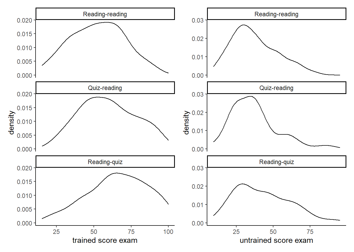

Looking at the first column (trained questions) we learn that quizzing shaves a good chunk of the lower (left) end of the distribution. With regard to the second column (untrained questions) it seems as if people from the middle of the distribution as pushed to the right.

d4 <- test %>% ggplot(aes(x=score_perc_New_exam)) +
  geom_density() +
  labs(x="new questions",
       y="density") +
  facet_wrap(vars(fct_relevel(learning_condition, "Reading-reading", "Quiz-reading", "Reading-quiz")), nrow = 3) +
  #coord_flip() +
  theme_classic()

d5 <- test %>% ggplot(aes(x=score_perc_General_exam)) +
  geom_density() +
  labs(x="generalizing questions",
       y="density") +
  facet_wrap(vars(fct_relevel(learning_condition, "Reading-reading", "Quiz-reading", "Reading-quiz")), nrow = 3) +
  #coord_flip() +
  theme_classic()

d4 + d5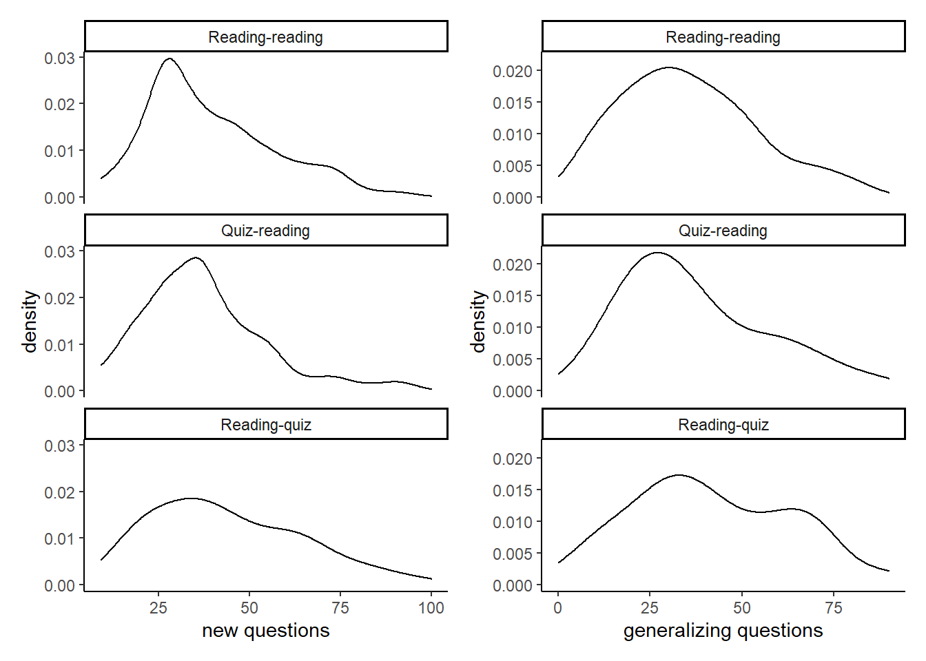

Zooming in on the untrained questions, we notice how the distributions flatten.

Now that we have a feel for the shape of the data, let us turn to inference.

The analysis

The researchers have followed the new standard for publishing experiments that use hypothesis tests. This new standard came about after so much research in psychology failed to replicate. In order to be published, many journals require so called p-values to be lower than 0.05. These values give the probability of seeing the data if there were no effect. If this is lower than 5%, then a study will be accepted. However, many researchers twisted and turned their data until they found an effect that is ‘significant’ in this artificial sense. Leaving out or imputing missing values as necessary may do the job as well. In response, researchers such as Latimier tell the journal in advance how much data they will collect, how they will handle missing values and how they will analyze the data. They also publish their data set, so that we can follow them along. This is all very laudable. However, hypothesis testing is rarely very interesting. We do not want to know if an effect is different from exactly zero. Instead, we want to know how big it is. Hence the Bayesian approach.

The question we focus on is the difference between Reading-reading and Reading-quiz, because this first condition is the one that most students use when they learn.

For a start we ask ourselves what we believe before we see the data. We have just seen the data of course, but that is okay now, because we will rely entirely on earlier research comparing re-reading and taking a test after reading. A meta-analysis from 2014 by Christopher Rowland included 159 studies (published and unpublished) that compared restudying (or re-reading, if you will) with testing after reading. The studies were roughly normally distributed with a mean of 0.5 and a standard deviation of 0.45.

Below we infer different priors from this meta-analysis and investigate the effect they have on the estimates. For reference, we first run a classical regression.

Frequentist inference

As input we use standardized versions of the score variables.

sd_pooled <- test %>% filter(learning_condition %in% c("Reading-reading", "Reading-quiz")) %>% 
      pull(scoreTotal_exam) %>% sd()

test <- test %>% group_by(learning_condition) %>% 
      mutate(scoreTotal_exam_st = scoreTotal_exam/sd_pooled) %>% 
      ungroup()

test_rr_rq <- test %>% filter(learning_condition != "Quiz-reading")

x <- lm(scoreTotal_exam_st ~ 1 + learning_condition, data = test_rr_rq)
summary(x)

## 
## Call:
## lm(formula = scoreTotal_exam_st ~ 1 + learning_condition, data = test_rr_rq)
## 
## Residuals:
##      Min       1Q   Median       3Q      Max 
## -2.20519 -0.67675 -0.07023  0.69399  2.28308 
## 
## Coefficients:
##                                   Estimate Std. Error t value Pr(>|t|)    
## (Intercept)                        3.17563    0.09876  32.154  < 2e-16 ***
## learning_conditionReading-reading -0.55800    0.13967  -3.995 9.28e-05 ***
## ---
## Signif. codes:  0 '***' 0.001 '**' 0.01 '*' 0.05 '.' 0.1 ' ' 1
## 
## Residual standard error: 0.9626 on 188 degrees of freedom
## Multiple R-squared:  0.07825,    Adjusted R-squared:  0.07335 
## F-statistic: 15.96 on 1 and 188 DF,  p-value: 9.276e-05

Compared to the re-reading group, the reading-quiz group performed about 0.558 standard deviations better. Compare this number to a direct calculation of the effect size.

# Calculate effect size step by step
mean_rr <- test %>% filter(learning_condition == "Reading-reading") %>% 
      pull(scoreTotal_exam) %>% mean()

mean_rq <- test %>% filter(learning_condition == "Reading-quiz") %>% 
      pull(scoreTotal_exam) %>% mean()

sd_pooled <- test %>% filter(learning_condition %in% c("Reading-reading", "Reading-quiz")) %>% 
      pull(scoreTotal_exam) %>% sd()

(mean_rr - mean_rq)/sd_pooled

## [1] -0.5580009

We have uncertainty about this estimate, which is represented by the standard error. It assumes that we calculated a sample mean (the effect size) that sits in a distribution of many sample means. The center of this sampling distribution is the true effect size. We don’t know where it sits however. We do not even know where our sample mean sits. But we know the standard deviation of this sampling distribution, which is estimated to be 0.14. The true effect size then probably isn’t more than 0.14 or possibly 0.28 removed from 0.558. This tells us it is probably not zero, but there is not much more we can say.

Bayesian inference

For more easily interpretable results we carry out a Bayesian analysis. We use different priors to demonstrate their effect on the estimates. The prior, to repeat, is what we believe before we see the data. In our case we have the results of 159 experiments on a range of subjects, with different populations and with different intervals between training and testing. It is up to the analyst to determine how to use these data.

Ideally, the meta-analysis would have provided us with a posterior distribution. That is, a distribution that tells us what we believe after seeing the 159 experiments. This posterior would represent for the present study the prior. Unfortunately, we do not have this posterior. But we do have estimates of the average and the standard deviation of the 159 experiments. We plug these as priors in a bayesian model.

# All studies combined
fit_ind_2 <-
  brm(data = test_rr_rq, 
      family = gaussian,
      scoreTotal_exam_st ~ 1 + learning_condition,
      prior = c(prior(normal(3, 2), class = Intercept),
                prior(normal(-0.5, 0.45), class = b)),
      iter = 2000, warmup = 1000, chains = 4, cores = 4,
      seed = 11,
      file = "fits/fit_ind_2")

plot(fit_ind_2)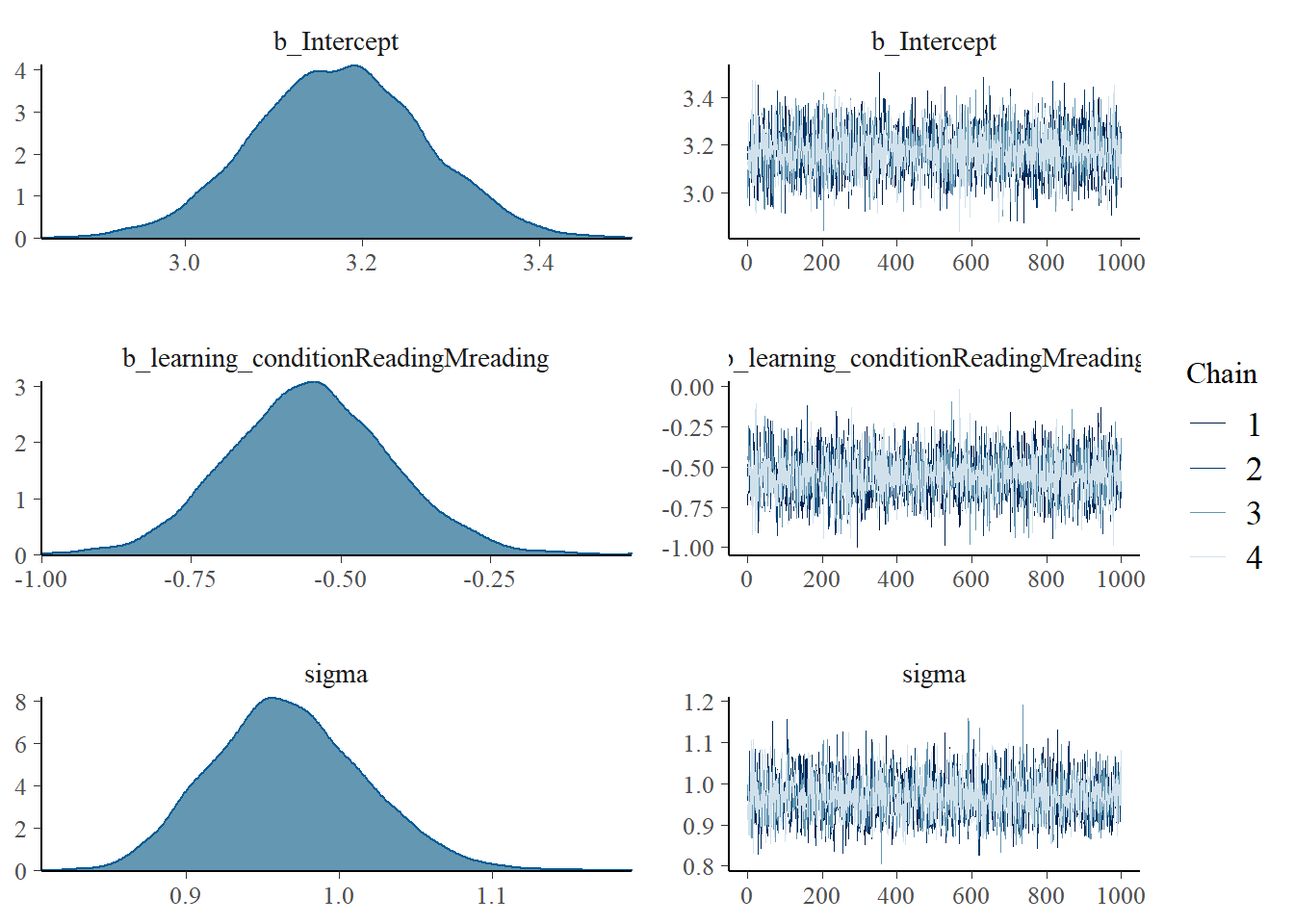

We marginalize over the posterior and get posterior distributions for all the parameters that we estimated. We care mainly about the second plot. It shows the probabilities of a specific effect size. This is not a sampling distribution. The density on the y-axis in this plot can actually be used to assign probabilities to outcomes!

Let us print the output.

print(fit_ind_2, digits=3)

##  Family: gaussian 
##   Links: mu = identity; sigma = identity 
## Formula: scoreTotal_exam_st ~ 1 + learning_condition 
##    Data: test_rr_rq (Number of observations: 190) 
## Samples: 4 chains, each with iter = 2000; warmup = 1000; thin = 1;
##          total post-warmup samples = 4000
## 
## Population-Level Effects: 
##                                   Estimate Est.Error l-95% CI u-95% CI  Rhat
## Intercept                            3.173     0.096    2.986    3.360 1.000
## learning_conditionReadingMreading   -0.552     0.133   -0.809   -0.285 1.001
##                                   Bulk_ESS Tail_ESS
## Intercept                             4319     3142
## learning_conditionReadingMreading     3898     3315
## 
## Family Specific Parameters: 
##       Estimate Est.Error l-95% CI u-95% CI  Rhat Bulk_ESS Tail_ESS
## sigma    0.967     0.050    0.876    1.068 1.000     4036     2778
## 
## Samples were drawn using sampling(NUTS). For each parameter, Bulk_ESS
## and Tail_ESS are effective sample size measures, and Rhat is the potential
## scale reduction factor on split chains (at convergence, Rhat = 1).

We notice that the estimate for the effect size has shrunk a little bit. This is the work of our prior. It had a mean of 0.5 and therefore we are sceptical of values that diverge from that estimate and pull the posterior estimate towards the mean we expect.

In contrast to the frequentist analysis we now have an idea about the value of the average effect size. We know where it is in the distribution and we can assign a probability to an interval around it. The standard error now helps us understand how wide this interval must be to assign a probability that we care about.

There is flexibility in setting this prior however. Rowland did a separate analysis on a subset of 92 studies that either provided feedback or had a training success rate over 75%. They had a mean of 0.66 and a standard deviation of 0.39. We run another model with these values.

# High exposure data set gives different prior
fit_ind_3 <-
  brm(data = test_rr_rq, 
      family = gaussian,
      scoreTotal_exam_st ~ 1 + learning_condition,
      prior = c(prior(normal(3, 2), class = Intercept),
                prior(normal(-0.66, 0.387), class = b)),
      iter = 2000, warmup = 1000, chains = 4, cores = 4,
      seed = 11,
      file = "fits/fit_ind_3")

print(fit_ind_3, digits=3)

##  Family: gaussian 
##   Links: mu = identity; sigma = identity 
## Formula: scoreTotal_exam_st ~ 1 + learning_condition 
##    Data: test_rr_rq (Number of observations: 190) 
## Samples: 4 chains, each with iter = 2000; warmup = 1000; thin = 1;
##          total post-warmup samples = 4000
## 
## Population-Level Effects: 
##                                   Estimate Est.Error l-95% CI u-95% CI  Rhat
## Intercept                            3.179     0.095    2.991    3.361 1.001
## learning_conditionReadingMreading   -0.569     0.132   -0.826   -0.311 1.001
##                                   Bulk_ESS Tail_ESS
## Intercept                             3982     2913
## learning_conditionReadingMreading     3683     2966
## 
## Family Specific Parameters: 
##       Estimate Est.Error l-95% CI u-95% CI  Rhat Bulk_ESS Tail_ESS
## sigma    0.968     0.049    0.879    1.071 1.001     3755     2984
## 
## Samples were drawn using sampling(NUTS). For each parameter, Bulk_ESS
## and Tail_ESS are effective sample size measures, and Rhat is the potential
## scale reduction factor on split chains (at convergence, Rhat = 1).

We see that this prior slighty moved the estimate upwards, but did not change the standard error by much.

Based on the data in the meta-analysis, Rowland calculated a confidence interval around the effect size of 0.5 with a width of 0.04. This is his estimate of where the true mean is. This is frequentist analysis, so it only means that the true mean is very close to 0.5. The standard error is so much smaller than the standard deviation of the effect sizes of the 159 studies, because we divide the standard deviation in the data by the square root of a huge amount of participants in the study.

Let us, for the moment, go with an enthusiastic interpretation that takes 0.5 as the mean of the prior distribution with standard deviation 0.04.

# Using the CI calculated by Rowland for the mean effect size
fit_ind_1 <-
  brm(data = test_rr_rq, 
      family = gaussian,
      scoreTotal_exam_st ~ 1 + learning_condition,
      prior = c(prior(normal(3, 2), class = Intercept),
                prior(normal(-0.5, 0.04), class = b)),
      iter = 2000, warmup = 1000, chains = 4, cores = 4,
      seed = 11,
      file = "fits/fit_ind_1")

print(fit_ind_1, digits=3)

##  Family: gaussian 
##   Links: mu = identity; sigma = identity 
## Formula: scoreTotal_exam_st ~ 1 + learning_condition 
##    Data: test_rr_rq (Number of observations: 190) 
## Samples: 4 chains, each with iter = 2000; warmup = 1000; thin = 1;
##          total post-warmup samples = 4000
## 
## Population-Level Effects: 
##                                   Estimate Est.Error l-95% CI u-95% CI  Rhat
## Intercept                            3.150     0.071    3.010    3.289 1.002
## learning_conditionReadingMreading   -0.504     0.039   -0.578   -0.429 1.001
##                                   Bulk_ESS Tail_ESS
## Intercept                             3281     3067
## learning_conditionReadingMreading     3597     2579
## 
## Family Specific Parameters: 
##       Estimate Est.Error l-95% CI u-95% CI  Rhat Bulk_ESS Tail_ESS
## sigma    0.965     0.050    0.873    1.069 1.000     4164     3118
## 
## Samples were drawn using sampling(NUTS). For each parameter, Bulk_ESS
## and Tail_ESS are effective sample size measures, and Rhat is the potential
## scale reduction factor on split chains (at convergence, Rhat = 1).

We see that this prior more aggressively tunes down the estimate of the effect size, as well as the estimate of the standard error.

plot(fit_ind_1, digits=3)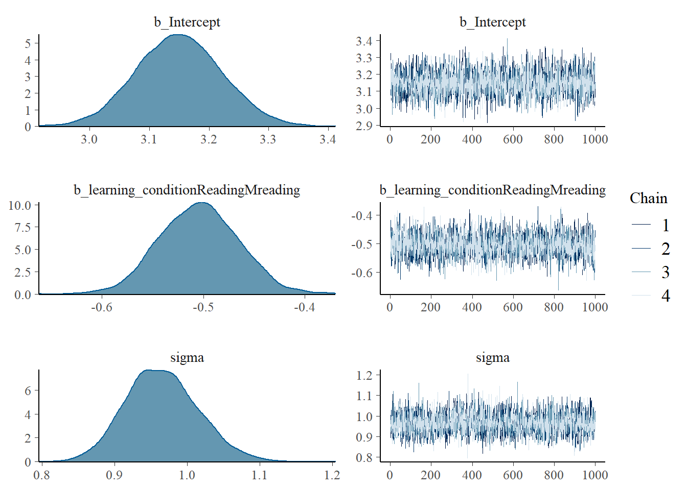

The posterior estimate of the effect size is now very tightly centered around 0.5. In this case, the prior was so narrow that the data did not have a chance to move it much. In general, high confidence in the prior means that it is tight, which means that in order for the data to move the estimate, it must be very tight itself or consist of many observations.

In this case, given the different topics in the 159 studies, the differences in study populations and time intervals, it would be unreasonable to set such a tight prior.

Instead, we should choose one of the first two priors. The second prior was based on a subset of studies with feedback or a training success rate above 75%. The present study actually did provide feedback and meets these criteria. However, initial success in training was well below 75%. The threshold criteria for inclusion seem arbitrary anyway.

In this case, the best prior then is the first one. This may seem as a let down, because results look very similar to those that the ordinary linear regression provided. There are benefits to the Bayesian approach though. First, the results are easier to interpret and do not require the frequentist dancing around assigning probabilities to outcomes. Second, Bayesian analysis takes advantage of cumulative research. As more studies come in, the standard deviation of the prior will shrink. Not as fast as calculating the standard error did, but it will get there eventually and more reasonably.