Do the Rich Influence Policy More than the Poor? (part 1)

A first look at the data

First, we load the data set and the packages that we will need for the data exploration.

library(foreign)
library(tidyverse)
library(haven)
library(naniar)
library(mice)
library(labelled)
library(ggthemes)
library(RColorBrewer)
library(patchwork)
library(reactable)

Schakel <- read_dta("C:/Users/Malorixverritus/Documents/R/website/datasets/Schakel 2019/Schakel_SER_Data.dta")

Schakel <- remove_labels(Schakel)

We note that the researchers were able to collect information on a total of 305 policy proposals that span 33 consecutive years, in the period 1979 - 2012.

Schakel %>% summarize(years = n_distinct(year))

## # A tibble: 1 x 1
##   years
##   <int>
## 1    33

Schakel %>% arrange(desc(year))

## # A tibble: 305 x 45
##       id  year  data survey spending  pass nocode  iall   i05   i10   i20   i30
##    <dbl> <dbl> <dbl>  <dbl>    <dbl> <dbl>  <dbl> <dbl> <dbl> <dbl> <dbl> <dbl>
##  1   250  2012    16      8        1     0     NA  43.1  44.8  44.1  43.0  42.2
##  2   251  2012    16      8        1     1     NA  48.2  37.7  40.3  44.9  48.5
##  3   252  2012    16      8        1     0     NA  76.6  78.5  78.0  77.3  76.6
##  4   253  2012    16      8        1     1     NA  51.6  62.4  57.4  49.2  43.9
##  5   254  2012    35      2        0     1     NA  80.6  77.2  79.1  81.8  83.4
##  6   255  2012    35      2        0     0     NA  10.5  16.1  15.1  13.5  12.0
##  7   256  2012    57      1        0    NA      1  47.5  45.5  45.6  46.0  46.6
##  8   257  2012    58      1        0     0     NA  63.1  57.9  58.7  60.3  62.1
##  9   258  2012    58      1        0     0     NA  38.8  30.7  31.8  34.1  36.7
## 10   259  2012    58      1        0     0     NA  30.9  18.7  20.7  25.0  29.6
## # ... with 295 more rows, and 33 more variables: i50 <dbl>, i70 <dbl>,
## #   i80 <dbl>, i90 <dbl>, i95 <dbl>, i10e10 <dbl>, i10e50 <dbl>, i10e90 <dbl>,
## #   i50e10 <dbl>, i50e50 <dbl>, i50e90 <dbl>, i90e10 <dbl>, i90e50 <dbl>,
## #   i90e90 <dbl>, men <dbl>, women <dbl>, iallv <dbl>, i10v <dbl>, i50v <dbl>,
## #   i90v <dbl>, iallnv <dbl>, i10nv <dbl>, i50nv <dbl>, i90nv <dbl>,
## #   unempt <dbl>, growtht <dbl>, debtt <dbl>, lrgovt <dbl>, unempt4 <dbl>,
## #   growtht4 <dbl>, debtt4 <dbl>, lrgovt4 <dbl>, question <chr>

This is a rich data set. The key variables are pass, which records whether a proposal passed or not within four years, and i05 up to i95, which tell us the percentage of support for a proposal per income group. The variable i05 refers to the policy preferences of people at the 5th percentile of the income distribution, for example. Between surveys, different income categories are used, so that the relative position of an individual on the income scale is estimated. A granular analysis of every tenth percentile of incomes is therefore not advisable, but the measure would seem good enough for comparing rich folks to poor ones.

Original answers were on an ordinal scale that captured levels of support for a policy. Ordinal scales differ from poll to poll however, so that it makes sense that responses have been collapsed into the binary categories “in favor” and “against”. We also note that the measure does not reflect the overall support for a policy of the income group, because those who answered ‘neutral’ are left out of the analysis. What the i10, i20, … i90 variables capture then is the percentage of support for a policy among those within an income group that have an opinion.

It has also been recorded whether people voted or not, so that i10v and i10nv are, respectively, voters and non voters at the 10th income percentile. The remaining variables are of lesser importance and will be described when they are used in the analysis.

Exploring key variables

A scatter plot of opinions of people at the 10th and 90th income percentiles shows that their preferences often align, but not so well that differences in support cannot explain variation in pass.

Schakel %>% ggplot(aes(x=i90, y=i10, color=factor(pass))) +
  geom_hline(yintercept=50) +
  geom_vline(xintercept=50) +
  geom_point() +
  scale_color_discrete(type=c("red","darkblue", "grey"),
                       labels=c("failure", "pass", "NA")) +
  theme_tufte() +
  labs(x="support at 90th percentile",
       y="support at 10th percentile",
       title = "Support for policies by income group and enactment",
       color="Enactment")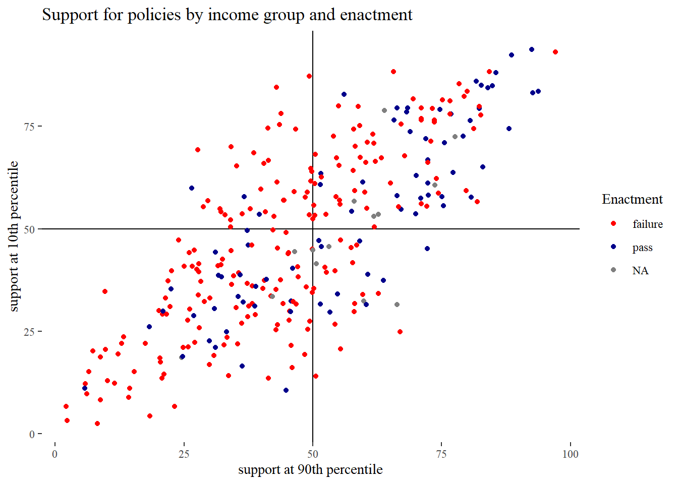

In order to get a feel for the nature of these proposals, we first show the proposals that low income people support more than the rich. To this end we display the 10 proposals from the top left rectangle, ordered by the gap in support between rich and poor. We then do the same for the bottom right rectangle, where the rich favor policies more than low income people.

Schakel %>% filter(i10>50 & i90<50) %>% 
  slice_max(order_by =(i10-i90), n=10) %>% 
  mutate(i10 = round(i10,0),
         i90 = round(i90, 0)) %>% 
  select(question, i10, i90) %>% 
  reactable(columns = list(
    question = colDef(name = "Question"),
    i90 = colDef(name = "90th income percentile support in %"),
    i10 = colDef(name = "10th income percentile support in %")
  ),)

Schakel %>% filter(i10<50 & i90>50) %>% 
  slice_max(order_by =(i90-i10), n=10) %>% 
  mutate(i10 = round(i10,0),
         i90 = round(i90, 0)) %>% 
  select(question, i90, i10) %>% 
  reactable(columns = list(
    question = colDef(name = "Question"),
    i90 = colDef(name = "90th income percentile support in %"),
    i10 = colDef(name = "10th income percentile support in %")
  ),)

Schakel %>% ggplot(aes(x=iallv, y= iallnv, color= factor(pass))) +
  geom_hline(yintercept=50) +
  geom_vline(xintercept=50) +
  geom_point() +
  scale_color_discrete(type=c("red","darkblue", "grey"),
                       labels=c("failure", "pass", "NA")) +
  theme_tufte() +
  labs(x="support among voters",
       y="support among non voters",
       title="Support for policies by voting and enactment",
       color="Enactment")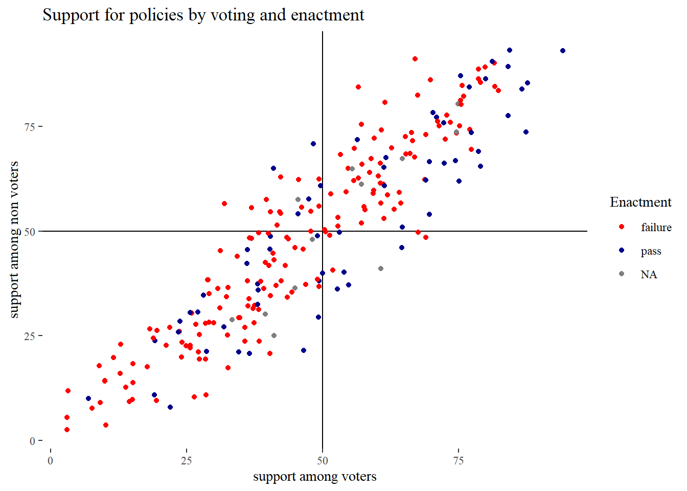

Missing data visualization

Before we carry on with the analysis we have to talk about missing data. We use the naniar package to handle missing data as well as to visualize it. For a first glance, we paint every cell in the data set that contains no information black.

vis_miss(Schakel, sort_miss = TRUE)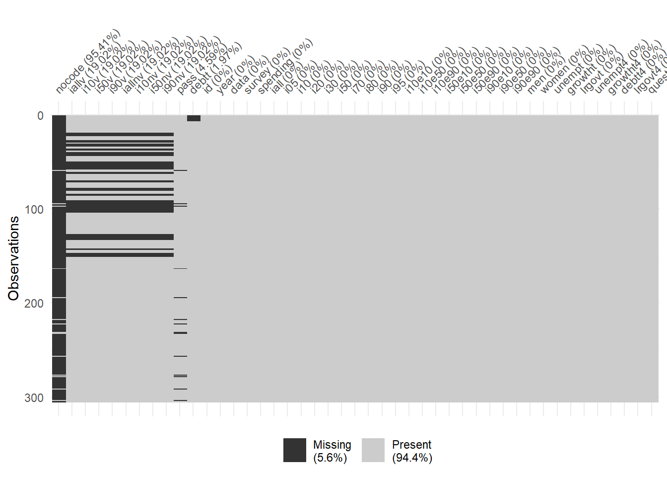

The column nocode is removed. It records the reason why pass is missing, and is therefore redundant. The eight columns to its right register whether subjects voted or not, specified for three income groups and all incomes (hence eight columns). Finally, there are missing values for pass itself (debt will not play a role in the analysis), which are crucial for the analysis. As the data set is arranged by year, we note that voting is missing more often in earlier years, whereas pass is missing more often for later years. Data are not missing randomly, then.

To put a number on the missing data, we produce a numeric summary that tells us that there are 58 polls that lack information on whether subjects voted or not and 14 that lack info on pass.

miss_var_summary(Schakel)

## # A tibble: 45 x 3
##    variable n_miss pct_miss
##    <chr>     <int>    <dbl>
##  1 nocode      291    95.4 
##  2 iallv        58    19.0 
##  3 i10v         58    19.0 
##  4 i50v         58    19.0 
##  5 i90v         58    19.0 
##  6 iallnv       58    19.0 
##  7 i10nv        58    19.0 
##  8 i50nv        58    19.0 
##  9 i90nv        58    19.0 
## 10 pass         14     4.59
## # ... with 35 more rows

We compare the percentage of support for a proposal between polls for which voting behavior is known or not. To this end, we first stick a copy of the data set underneath, of which the values inform us whether data are missing or not and then produce some graphs.

Schakel <- Schakel %>% select(-nocode)

Schakel_NA <- Schakel %>% 
  bind_shadow()

p1 <- Schakel_NA %>% ggplot(aes(x=iall, color = iallv_NA)) +
  geom_density() +
  scale_color_discrete(type=c("darkgreen", "grey"),
                       labels=c("data", "no data")) +
  theme_tufte() +
  labs(x="support all income groups",
       color="Voting behavior")

p2 <- Schakel_NA %>% ggplot(aes(x=i90, color = iallv_NA)) +
  geom_density() +
  scale_color_discrete(type=c("darkgreen", "grey"),
                       labels=c("data", "no data")) +
  theme_tufte() +
    labs(x="support 90th percentile income",
       color="Voting behavior")

p3 <- Schakel_NA %>% ggplot(aes(x=i10, color = iallv_NA)) +
  geom_density() +
  scale_color_discrete(type=c("darkgreen", "grey"),
                       labels=c("data", "no data")) +
  theme_tufte()+
    labs(x="support 10th percentile income",
       color="Voting behavior")

p1 + p3 + p2 + plot_layout(ncol=1)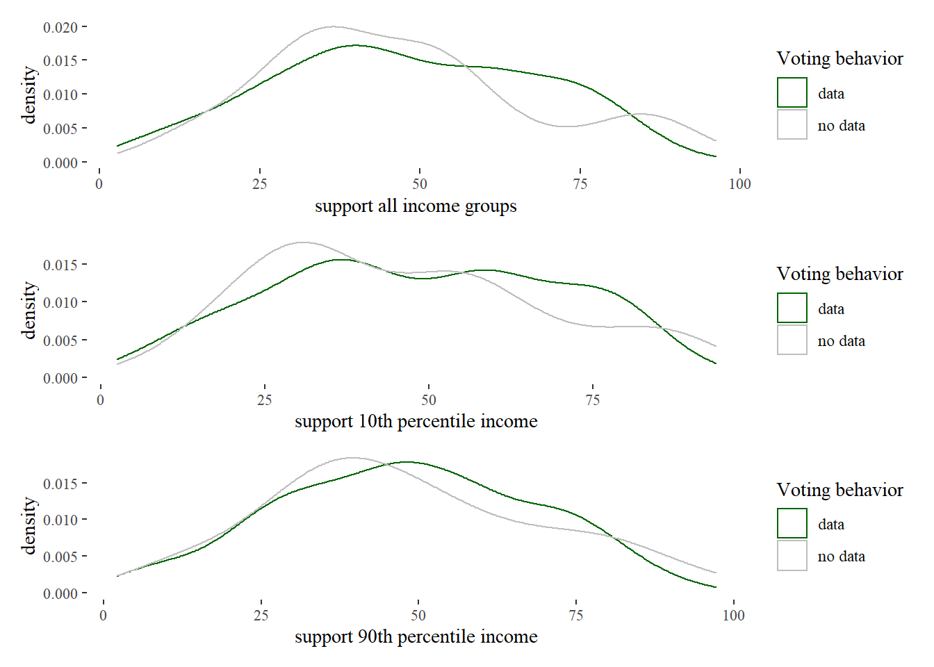

Whether their voting behavior is recorded or not, the preferences of all subjects have a similar distribution. The same is true for low income and for high income voters. However, both groups tend to be slightly less supportive of a proposal in polls for which it was not recorded whether a person votes in elections or not.

The final variable for which missing values are relevant for the analysis is pass. This variable measures whether a proposal is passed or not. We want to know if support for proposals for which it is unknown if it was passed, differs from proposals for which we know if it passed or not.

p4 <- Schakel_NA %>% ggplot(aes(x = iall)) +
  geom_histogram(aes(y = ..density..), fill="red3", binwidth = 5) +
  facet_wrap(~ pass_NA) +
  labs(x="support all individuals") +
  theme_tufte()

p5 <- Schakel_NA %>% ggplot(aes(x = iall, y = pass_NA)) +
  geom_boxplot()+
  labs(x="support all individuals") +
  theme_tufte()

p6 <- Schakel_NA %>% ggplot(aes(x = i10)) +
  geom_histogram(aes(y = ..density..), fill="red3", binwidth = 5) +
  facet_wrap(~ pass_NA) +
  labs(x="support 10th percentile") +
  theme_tufte()

p7 <- Schakel_NA %>% ggplot(aes(x = i10, y = pass_NA)) +
  geom_boxplot()+
  labs(x="support 10th percentile") +
  theme_tufte()

p8 <- Schakel_NA %>% ggplot(aes(x = i90)) +
  geom_histogram(aes(y = ..density..), fill="red3", binwidth = 5) +
  facet_wrap(~ pass_NA) +
  labs(x="support 90th percentile") +
  theme_tufte()

p9 <- Schakel_NA %>% ggplot(aes(x = i90, y = pass_NA)) +
  geom_boxplot()+
  labs(x="support 90th percentile") +
  theme_tufte()

p4 + p5 +p6 + p7 + p8 + p9 + plot_layout(ncol=2)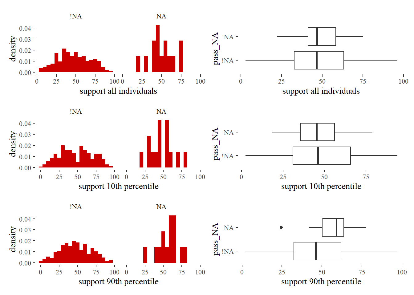

We note that if it was not recorded if a proposal was passed or not, high income people tend to be more supportive compared to proposals for which the outcome was recorded. We furthermore note that none of the proposals with a missing pass outcome was about spending.

Schakel_NA %>% filter(pass_NA =="NA") %>% 
  count(spending)

## # A tibble: 1 x 2
##   spending     n
##      <dbl> <int>
## 1        0    14

With regard to information on income of subjects, we observe that no data are missing. This suggests that only polls that provided income data have been included in the sample. It is impossible to determine whether this has led to a bias in the selection of types of policy proposals.

What to do about missing data

Simply throwing away rows with missing data can seriously bias results. Even if values were missing due to some random process (and it is hard to imagine what that would even look like), throwing away data would increase the standard error, so that it is harder to generalize from the data.

The proper way to proceed is to impute missing values. That is, to come up with estimates of missing values based on the data. To this end, simple imputations like taking the mean or the lowest value of a variable heavily bias the data. Instead, one ought to fill in missing values with a regression model. Better still is to not only model the uncertainty as the error term in a regression model, but to also model the uncertainty in the parameters of the model. This approach is know as multiple imputation. There are actually several values generated per empty cells and hence many data sets. In our case 5.

Schakel_imp <- mice(Schakel, m = 5, print = FALSE)

In a bayesian framework, these data sets will all generate posteriors from which samples are drawn by software. These samples can subsequently be thrown together to form a so called posterior, which is a distribution that assigns probabilities to the quantity that we care about. This posterior will not just incorporate the error of the regression model that mice uses for the imputation, but also the uncertainty in the estimates of this model (for every parameter there are five estimates). Generating these posteriors will be part of the analysis, to which we turn next.