Causal Inference 3: Synthetic Control
So far, we first saw that fixed effects was able to get rid of confounders that did not change over time. We then noted that difference in differences designs could do better, as they got rid of confounders that changed over time parallel to the whole control group. Rather than assume that the path of the counterfactual has the slope of the control, the synthetic control method attempts to estimate this path. This is more progress still.
The method was introduced by Alfonso Abadie in 2003 and took off in the area of policy research after packages became available in 2010. One of it’s main strengths is that it offers insights into causal effects in a way that is easy to follow for policymakers. The basic idea can be grasped without any understanding of inferential statistics. Specifically, the Central Limit Theorem plays no role whatsoever, which is typically the main culprit behind confusion about inferential results.
We will first describe the inner workings of the model in a technical note. The basic idea expressed here is that we compare a treatment unit (often a country) to similar units (perhaps countries on the same continent). These controls are called the donor pool. From them, the method select bits and pieces to create a fake version of the treatment unit, in a Frankenstein fashion. This counterfactual treatment unit is then pushed into the future. The difference of its trajectory with that of the actual treatment unit is said to be caused by the intervention.
After the technical exposition, we apply the method to the case of economic growth in Sub-Saharan Africa, where we wonder if becoming a democracy boosts GDP. Finally, we briefly look at some extensions of the synthetic control method. This is a very active area of research, with several attempts to not only extend the method in several ways but also to connect it to other approaches to causal inference, such as matching, latent factor models and difference in differences. We apply one of these extensions to our case study and reflect on the hard questions about causal inference it poses.
Technical note
The Synthetic Control Method
Let’s set up some notation so that we can delve into the inner workings of the synthetic control method. We let
Here
The first step is to choose a bunch of characteristics that are unaffected by the intervention. The characteristics for the intervention unit are collected in a vector
To get a better picture of what goes on under the square root sign, we assume that V is diagonal. Multiplying V with the vector to its right results in a vector where the weights on the diagonal of V are multiplied with the vector component of the same row on its right. Multiplying the transpose of
Now, we could set the weights for the features by hand. But that would be too arbitrary. A better way, among many ways, would be to calculate (using cross validation) values of V that make the squared difference in the outcome of interest between the treatment unit and the donor pool - in the pre-treatment periods - as small as possible.
Unlike for the case of the W of the synthetic control method, the weights W from the regression are not necessarily between 0 and 1. Having negative weights would mean that we subtract a countries’ outcome, which would bring us outside of the support - that is, outside the realm of events that happened. But we want to construct our synthetic counterfactual by adding up events that happened. It we subtract part of the outcome of Nigeria from that of Botswana and call the result our counterfactual, we may be dealing with an outcome that could never come about in reality. Using regression weights would therefore be less convincing.
The Data
The intuitive strenth of the synthetic control method shines when it is applied. We therefore replicate a study by Wittels and De Kadt from 2016 on the role of democracy in promoting economic growth in sub sharan Africa. The data are available here.
Let’s first check which Sub-Saharan countries became democratic in what year. (South Africa is not included, because it is too different from the other countries.) We use the handy panelView package to visualize the answer to this question.
library(tidyverse)
library(haven)
library(tidysynth)
library(panelView)
require(gridExtra)

## Data
load("C:/R/politics/democracy_growth_sub_sahara/afripanel_wdk_final.RData")


# How does it know dem is treatment? Because first var on RHS is always the treatment
plot1 <- panelView(lngdpmad ~ dem + lngdpmadlag + lngdpmadlag2 + lngdpmadlag3 + lngdpmadlag4 +
            civwar + ki + civwarend + openk + pwt_xrate + pwt_xrate_lag1 + pwt_xrate_lag2 +
            pwt_xrate_lag3,
          data = afripanel,
          index = c("Country","year"),
          xlab = "Year", ylab = "Country",
          pre.post = T)
plot1 +
theme(axis.text.x = element_text(angle = 90, vjust = 0.5, hjust=1))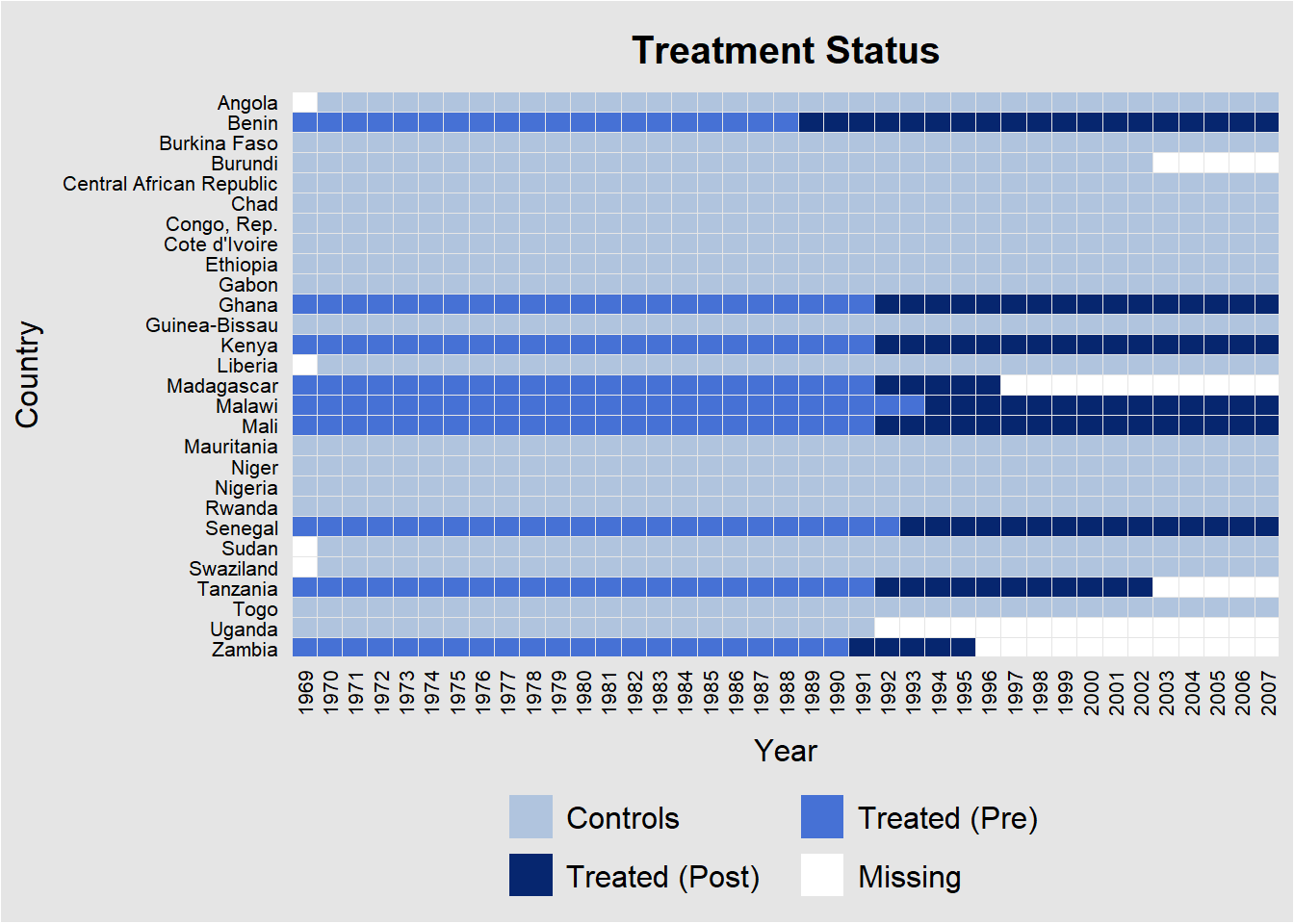
We see that nine countries became democratic after 1990. The other countries are selected because they are supposed to provide a good control group. This is a researcher degree of freedom in the synthetic control method. The researcher is supposed to pick control units that are similar. Otherwise, if there are not too many covariates, the model may pick up on commonalities in units that move on a very different trajectory.
Just so that we know what we are talking about, we plot the average GDP per capita in dollars over the time period. (I will not question the reliability of these data here.)
# plot mean gdp1 over time (what is gdp2?)
afripanel %>%
group_by(Country) %>%
summarize(gdp1 = mean(gdp1, na.rm=T), gdp2 = mean(gdp2, na.rm=T)) %>%
mutate(Country = fct_reorder(Country, gdp1)) %>%
ggplot(aes(Country, gdp1, fill=Country)) +
geom_col(show.legend = F) +
coord_flip()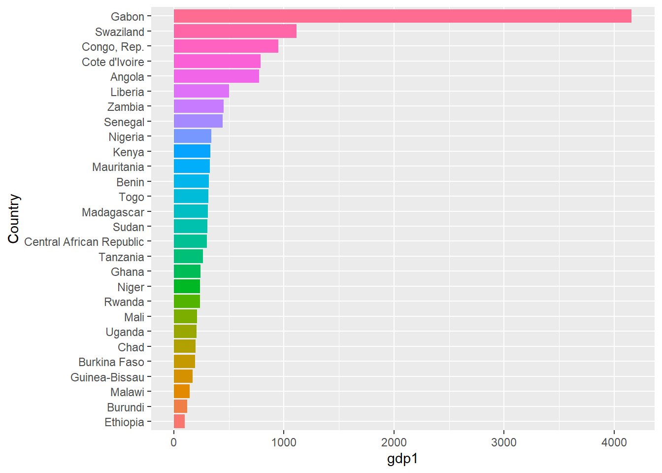 Many countries have average incomes of less than a dollar a day in this period, unless they sit on valuable resources.
We next plot trends in GDP over time for states that became democratic and the control states.
library(ggsci)
afripanel %>%
filter(Country != "Gabon") %>%
ggplot(aes(x=year, y=gdp1, group=Country, color=factor(dem))) +
geom_line(size=1) +
scale_color_npg() 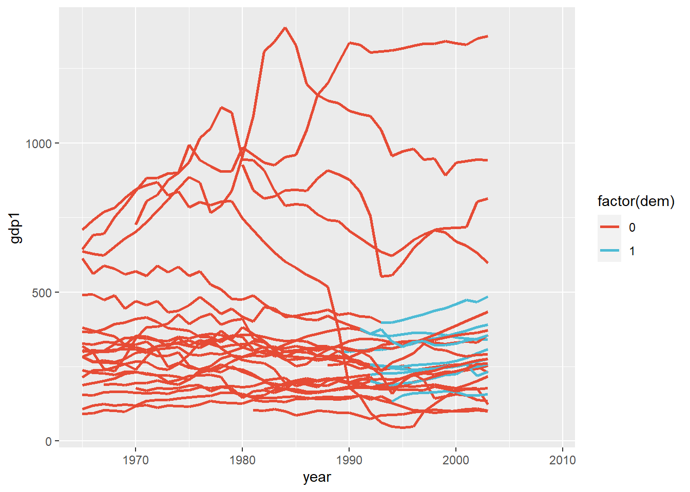 There seems to be some upward movement for the democratic states (in blue), but the controls are moving up as well. We hope that the synthetic control method can tease apart what part of the upward trend is caused by becoming democratic.
Before the authors turn to investigating whether democracy boosts GDP in all Sub-Saharan democracies, they first focus on the case of Mali. We will reproduce their analysis using the tidysynth package.
dems <- afripanel %>% filter(dem=="1" & !WBCode=="MLI") %>%
  distinct(WBCode) %>%
  pull(WBCode)

subsah_out <-

  afripanel %>%

  filter(!WBCode %in% dems) %>%

  # initial the synthetic control object
  synthetic_control(outcome = lngdpmad, # outcome
                    unit = WBCode, # unit index in the panel data
                    time = year, # time index in the panel data
                    i_unit = "MLI", # unit where the intervention occurred
                    i_time = 1991, # time period when the intervention occurred
                    generate_placebos=T # generate placebo synthetic controls (for inference)
  ) %>%

  # Generate the aggregate predictors used to fit the weights

  # average log income, retail price of cigarettes, and proportion of the
  # population between 15 and 24 years of age from 1980 - 1988
  generate_predictor(time_window = 1975:1990,
                     lag1 = mean(lngdpmadlag, na.rm=T),
                     lag2 = mean(lngdpmadlag2, na.rm=T),
                     lag3 = mean(lngdpmadlag3, na.rm=T),
                     lag4 = mean(lngdpmadlag4, na.rm=T),
                     ki = mean(ki, na.rm=T),
                     openk = mean(openk, na.rm=T),
                     civwar = mean(civwar, na.rm=T),
                     civwarend = mean(civwarend, na.rm=T),
                     pwt_xrate = mean(pwt_xrate, na.rm=T),
                     pwt_xrate_lag1 = mean(pwt_xrate_lag1, na.rm=T),
                     pwt_xrate_lag2 = mean(pwt_xrate_lag2, na.rm=T),
                     pwt_xrate_lag3 = mean(pwt_xrate_lag3, na.rm=T),
                     wbank = mean(wbank, na.rm=T),
                     wbank_lag1 = mean(wbank_lag1, na.rm=T),
                     wbank_lag2 = mean(wbank_lag2, na.rm=T),
                     imfadj = mean(imfadj, na.rm=T),
                     imfadj_lag1 = mean(imfadj_lag1, na.rm=T),
                     imfadj_lag2 = mean(imfadj, na.rm=T)
                     ) %>%

  # Generate the fitted weights for the synthetic control
  generate_weights(optimization_window = 1975:1991, # time to use in the optimization task
                   margin_ipop = .02,sigf_ipop = 7,bound_ipop = 6 # optimizer options
  ) %>%

  # Generate the synthetic control
  generate_control()


subsah_out %>% plot_trends() + xlim(1975,2008)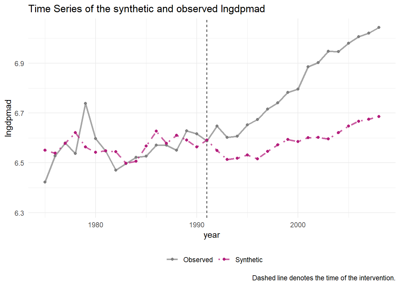
We here reproduce the graph that the authors published in their journal article. Before 1991, when Mali became democratic, we notice that the synthetic control matches the development of Mali quite closely. This suggests that we can reproduce the dynamics of GDP in Mali and have created a flexible control. The graph is cut off in 1975, because for this period most variables are available. However, we saw in the panelView plots that data for at least some of the variables go all the way back to 1969. Let’s plot the entire period and see what happens.
subsah_out %>% plot_trends()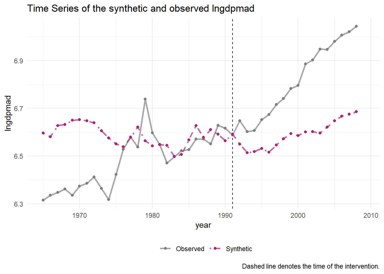 The full picture looks a lot less convincing. It suggests we can reproduce the development of Mali’s GDP well between 1975 and 1991, but when we extrapolate back in time, the synthetic control diverges. If so, why should we trust the synthetic control if we extrapolate forward in time?
This demonstrates the main problem for a synthetic control analysis. It must be convincing that the model didn’t overfit. If it did overfit, we cannot confidently extrapolate back in time or forward in time (the latter case generates the counterfactual). The model above is, judged by the picture, certainly not convincing. The authors provide a second specification though, in which they leave out Ethopia and Benin so that they can include the difference between exports and imports as a predictor.
# Without Ethopia and Sudan
subsah_out_imex <-
afripanel %>% filter(!WBCode %in% c("SDN", "ETH") & !WBCode %in% dems) %>%
# initial the synthetic control object
synthetic_control(outcome = lngdpmad, # outcome
unit = WBCode, # unit index in the panel data
time = year, # time index in the panel data
i_unit = "MLI", # unit where the intervention occurred
i_time = 1991, # time period when the intervention occurred
generate_placebos=T # generate placebo synthetic controls (for inference)
) %>%
# Generate the aggregate predictors used to fit the weights
# average log income, retail price of cigarettes, and proportion of the
# population between 15 and 24 years of age from 1980 - 1988
generate_predictor(time_window = 1975:1990,
lag1 = mean(lngdpmadlag, na.rm=T),
lag2 = mean(lngdpmadlag2, na.rm=T),
lag3 = mean(lngdpmadlag3, na.rm=T),
lag4 = mean(lngdpmadlag4, na.rm=T),
ki = mean(ki, na.rm=T),
openk = mean(openk, na.rm=T),
civwar = mean(civwar, na.rm=T),
civwarend = mean(civwarend, na.rm=T),
pwt_xrate = mean(pwt_xrate, na.rm=T),
pwt_xrate_lag1 = mean(pwt_xrate_lag1, na.rm=T),
pwt_xrate_lag2 = mean(pwt_xrate_lag2, na.rm=T),
pwt_xrate_lag3 = mean(pwt_xrate_lag3, na.rm=T),
eximdiff = mean(eximdiff, na.rm=T),
eximdiff_lag1 =mean(eximdiff_lag1, na.rm=T),
eximdiff_lag2 =mean(eximdiff_lag2, na.rm=T),
wbank = mean(wbank, na.rm=T),
wbank_lag1 = mean(wbank_lag1, na.rm=T),
wbank_lag2 = mean(wbank_lag2, na.rm=T),
imfadj = mean(imfadj, na.rm=T),
imfadj_lag1 = mean(imfadj_lag1, na.rm=T),
imfadj_lag2 = mean(imfadj, na.rm=T)
) %>%
# Generate the fitted weights for the synthetic control
generate_weights(optimization_window = 1975:1991, # time to use in the optimization task
margin_ipop = .02,sigf_ipop = 7,bound_ipop = 6 # optimizer options
) %>%
# Generate the synthetic control
generate_control()
subsah_out_imex %>% plot_trends() 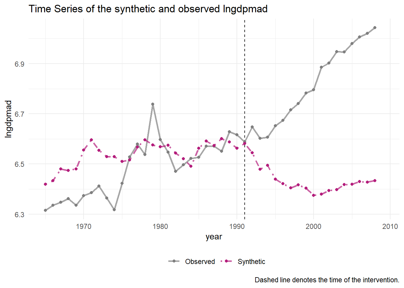 Although not perfect, this model is a more convincing.
We can compare the regression weights for the model that predicted GDP in Mali with those of the model that predicted GDP for the synthetic control and observe that they are reasonably similar.
subsah_out_imex %>% grab_balance_table()## # A tibble: 21 x 4
## variable MLI synthetic_MLI donor_sample
## <chr> <dbl> <dbl> <dbl>
## 1 civwar 0.0625 0.0845 0.188
## 2 civwarend 0.0625 0.0369 0.0257
## 3 eximdiff 0.350 0.0925 0.0133
## 4 eximdiff_lag1 0.371 0.0988 0.0284
## 5 eximdiff_lag2 0.419 0.102 0.0261
## 6 imfadj 0.125 0.127 0.0772
## 7 imfadj_lag1 0.0625 0.123 0.0662
## 8 imfadj_lag2 0.125 0.127 0.0772
## 9 ki 21.6 19.2 21.9
## 10 lag1 6.54 6.56 6.98
## # ... with 11 more rowsThey are a lot better than for the donor sample as a whole at least.
Another aspect of interest is to investigate the two types of weights that are estimated.
# two types of weights
subsah_out_imex %>% plot_weights()
The weight on the donor pool show that Burundi, Togo and Burkina Faso are most similar. I know very little about african economic development, but the latter two countries are very close to Mali geographically, which gives some confidence.
As to the weights on the variables, we note that being in a civil war has the biggest impact, which also makes a lot of sense.
Let’s turn next to the uncertainty of our causal estimate. In the original version of synthetic control there is only one intervention unit, so we have no variation on which to build standard errors. Moreover, in the article on difference in differences, we noted that the standard error on the interaction term in the regression model doesn’t encapsulate all the uncertainty we care about. Our uncertainty concerns the generation of the synthetic counterfactual. How good is it really? We have of course no benchmark against which to test this: by definition, a counterfactual didn’t happen. So it seems we’re stuck.
One way to proceed, taken by Abadie, is to take not Mali, but Burundi as the treatment unit and all other countries (including Mali) as the control, and run the model. This produces a counterfactual for Burundi, that should actually match it after 1991 (the treatment period for Mali) because Burundi did not become democratic. We repeat this analysis for all the other countries. If the method doesn’t overfit too much, Mali should be an outlier. (In this case along with other countries that became democratic at this time.)
The plot below shows the result of this procedure.
subsah_out_imex %>% plot_placebos(prune = FALSE)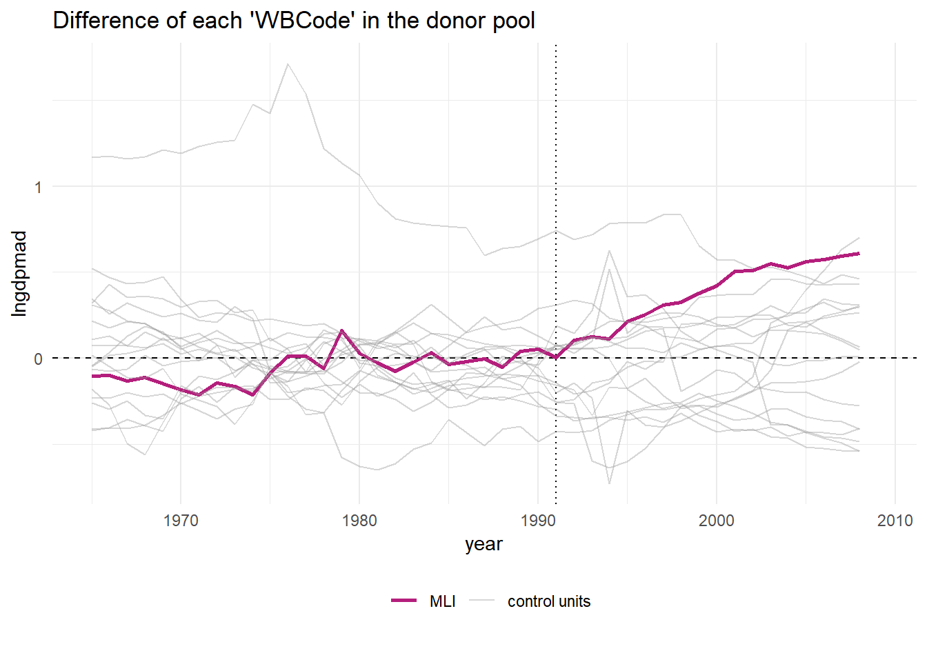 In this picture, we see the difference between the actual GDP in a country minus the counterfactual synthetic control for that country. Before 1991 this number should be zero for all countries in the plot, because none are democratic. After 1991 it should be zero for all countries excepr for Mali (we removed all democracies other than Mali). Most countries are close to zero, but there are outliers where the synthetic control fails to match pre-treatment GDP. For these countries the synthetic control is a bad model. The reason is probably that these countries lie outside the support. That is, values on their covariates or dependent variables are higher (or lower) than in any of the other countries, so that the relation in these ranges cannot be replicated by putting together bits and pieces of the other countries.
Below, we therefore remove countries for which the pre-treatment fit was bad.
subsah_out_imex %>% plot_placebos()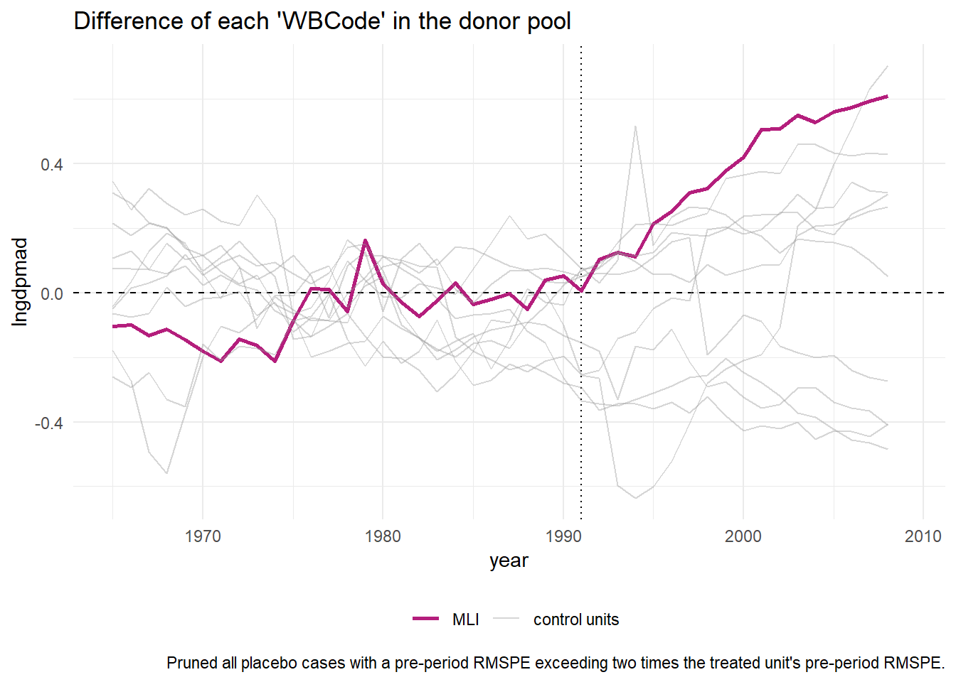 This leaves 12 countries, which show that Mali is an outlier in terms of it’s post-treatment distance to its counterfactual. This gives more confidence in the model and its suggestion that becoming a democracy was the cause of GDP growth in Mali.
But why pick Mali and not Benin or one of the other countries that became democratic around 1991? If only Mali outperformed its counterfactual, while the other democracies didn’t, would we say that democracy boosts GDP in some countries and not in others? That is what the authors of the original paper are inclined to say after they repeat the above analysis for every individual democracy in the data set.
But wouldn’t it be at least as reasonable to doubt the role of democracy if it sometimes fails and sometimes succeeds? Why not treat all democracies as one group, and compare them with comparable non-democratic countries? That is what can now be accomplished with extensions of the synthetic control method.
Developments in the Synthetic Control Method
Let’s back up for a moment and talk about advances in the synthetic control method, before we go on to answer the question about democracy and GDP growth in general in Sub-Saharan Africa. These advances move in several directions, which is exciting, but can also be confusing as it is not always clear how the methods relate to each other. The dust is yet to settle.
Let me briefly mention a couple of directions. There is work that addresses cases where there are multiple outcome measures. Other approaches address cases where the treatment unit is on the edge of the convex hull of the data, so that no proper comparison units exist. And then there are approaches that apply the method to situations where there are multiple treatment units. A prominent version is the so called synthetic difference in differences method. It ties together several strains of causal inference research and is therefore useful to discuss in a little more detail.
By rewriting the synthetic control model, it can be shown that synthetic control is a type of ‘vertical’ regression, in the sense that the controls are regressed on the treatment (‘horizontal’ would be if we regress through time). With the twist that weights between 0 and 1 are involved. We say that the regression is weighted then.
Rewriting the difference in differences model shows that it can be written as a vertical regression as well, but with fixed unit effects and fixed time effects added in. But this time the regression is unweighted.
Synthetic difference in differences, you guessed it, is the difference in differences regression model multiplied by the weights parameter of synthetic control. On top of that it also has weights for trends through time. Another difference compared to the synthetic control method is that the weights on the control units are estimated with a ridge regression, so that there is a penalty term. In estimating the weights for time trends there is no penalty term, because simulations show that better results are achieved if the model is allowed to weigh recent events more heavily. A penalty term may eliminate these.
There is also an R package for implementing the approach, but the method requires that the intervention takes place at the same time for all treatment units, which is not the case for our data.
We therefore turn to the gsynth package, which stands for generalized synthetic control. It treats finding the counterfactual as a missing data problem. It first uses the control group data and fits a model to it which reduces the covariates to a number of latent factors. The treatment units are then projected onto the space spanned by this lower rank matrix. Each treatment thereby gets a factor loading. After adding these to the matrix, the counterfactuals are imputed as if they were missing data. For more details, read the article here.
We now apply this method to all the democracies in the data set to check democracy’s causal impact on GDP.
library(gsynth)
library(Rcpp)
library(foreach)
library(doParallel)
library(lfe)
library(abind)
library(GGally)

afripanel_NA <- na.omit(afripanel)

system.time(
  out <- gsynth(lngdpmad ~ dem + lngdpmadlag + lngdpmadlag2 + lngdpmadlag3 + lngdpmadlag4
                + civwar + ki + civwarend + openk + pwt_xrate + pwt_xrate_lag1 + pwt_xrate_lag2 +
                pwt_xrate_lag3,
                data = afripanel_NA,
                index = c("Country","year"),
                force = "two-way",
                CV = TRUE,
                r = c(0, 5),
                se = TRUE,
                inference = "parametric",
                nboots = 1000,
                parallel = TRUE)
)## Some treated units has too few pre-treatment periods.
## They will be automatically removed.
## Parallel computing ...
## Cross-validating ...
## r = 0; sigma2 = 0.00354; IC = -5.44752; MSPE = 0.00198
## r = 1; sigma2 = 0.00283; IC = -5.04441; MSPE = 0.00197*
## r = 2; sigma2 = 0.00233; IC = -4.64795; MSPE = 0.00259
## r = 3; sigma2 = 0.00194; IC = -4.27520; MSPE = 0.00323
## r = 4; sigma2 = 0.00167; IC = -3.90085; MSPE = 0.00482
## r = 5; sigma2 = 0.00152; IC = -3.49821; MSPE = 0.00862
##
## r* = 1
##
##
Simulating errors ...
Bootstrapping ...
##
list of removed treated units: Tanzania## user system elapsed
## 1.00 0.30 8.87plot(out)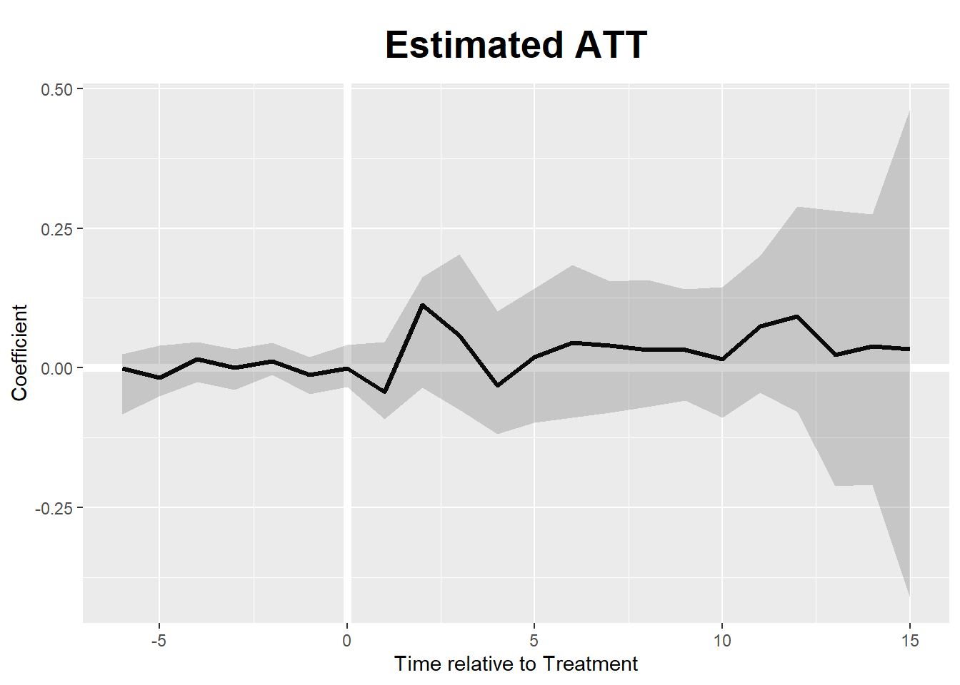 Given this plot, we are not sure at all that democracy on average plays a role for good in terms of boosting GDP in Sub-Saharan Africa. Given the (bootstrap based) uncertainty band, it may hamper growth as well.
This is an interesting state of affairs. If we believe the original synthetic control method, it takes some intellectual gymnastics to reconcile it’s results for individual cases with the result in the plot above. It is of course possible that democracy is the cause of GDP growth in some countries while it slows down growth in others. Economies are very different. Maybe the level of trade or resource exploitation interacts in some way with democratic institutions. But the burden may be on those who claim distinct effects to show these interactions exist.
Moreover, the confidence in the causal claim in individual cases is diminished by the indirect nature of the placebo inference method. In the case of Mali, the placebo trials on the controls that we demonstrated were not all that convincing anyway, because the pre-treatment fit was not great.
In this case, the causal effect of democracy on GDP in Mali may have been due to researcher degrees of freedom. The placebo methods shows that the counterfactual for Mali is likely noisy, given the imperfect pre-treatment fit, which is also true for the other democracies. Noise means variation and the fact that the effect in Mali is the greatest of all countries suggests that it was not the most representative case. Noise in the data and researcher degrees of freedom remain a dangerous combination. The synthetic control method is not exempt from this threat.
Edi Terlaak
I like to tell stories about statistics.